Visualization · Plotting

Plotting — the front door

There is exactly one entry point for turning a trajectory into a figure: to_plot_spec. Every common view — a time series, a phase portrait, a spacetime image, a delay embedding, a spatial-field movie — comes out of it, and its sibling .plot(...) builds the spec and renders it in a single call. Learn this one method and you can draw everything the library produces.

import tsdynamics as ts

traj = ts.systems.Lorenz(ic=[1.0, 1.0, 1.0]).integrate(final_time=100.0, dt=0.01)

traj.plot()                         # render immediately (auto-dispatched)
spec = traj.to_plot_spec()          # …or keep the spec, tweak it, then render

The two forms differ only in when they render. to_plot_spec(...) returns the backend-agnostic PlotSpec so you can chain tweaks (.relabel, .recolor, .grid, …) and choose an output; .plot(...) is the same thing plus an immediate render. Everything below is written against to_plot_spec — swap in .plot whenever you just want a picture.

Plot straight from a system

system.to_plot_spec(...) / system.plot(...) accept integration keywords too (final_time, dt, ic, method, …) — the system integrates first, then builds the spec, splitting the two kinds of keyword for you:

ts.systems.Rossler(ic=[1.0, 1.0, 1.0]).plot(final_time=200, dt=0.05,
                                             components=["x", "y"])

Auto-dispatch: the kind follows the components

With no kind=, to_plot_spec picks the semantic kind from how many components you are drawing — the natural view for that dimensionality:

Components drawn	Auto kind	What you get
1	TIME_SERIES	the channel against time
2	PHASE_PORTRAIT_2D	a 2-D orbit on equal axes
3	PHASE_PORTRAIT_3D	a 3-D attractor
4 or more	SPACETIME	a component-vs-time field image

traj = ts.systems.Lorenz(ic=[1.0, 1.0, 1.0]).integrate(final_time=100, dt=0.01)

traj.to_plot_spec().kind                          # → 'phase_portrait_3d'  (all 3)
traj.to_plot_spec(components="x").kind             # → 'time_series'        (1)
traj.to_plot_spec(components=["x", "z"]).kind      # → 'phase_portrait_2d'  (2)

The 4+-case is deliberate: a high-dimensional flow (a Lorenz-96 lattice) reads as a spacetime field, never as a misleading 3-D portrait of its first three coordinates. A discrete-map orbit is drawn with a SCATTER mark (a point sequence), not a joined line, because successive iterates are not continuous.

You override the auto-dispatch with kind= (any member of the closed PlotKind vocabulary, plus the "delay" and "field" recipes) and you pick which channels with components=. The rest of this page walks every kind.

---

Time series

One or more components against time. With kind=None you get this whenever a single component is selected; passing kind="time_series" overlays every selected component as its own line (a legend appears automatically for two or more).

ros = ts.systems.Rossler(ic=[1.0, 1.0, 1.0]).integrate(final_time=200.0, dt=0.05)

# all three components, x(t) / y(t) / z(t), overlaid with a legend
ros.to_plot_spec(kind="time_series").save("rossler-ts.pdf")

# just one channel
ros.to_plot_spec(components="x").save("rossler-x.pdf")

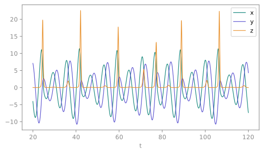
The Rössler system's three components overlaid via kind="time_series". The smooth x/y oscillation and the sharp periodic z-spikes (the reinjection kicks) are the signature of the Rössler folding — one legend, one set of axes.

Reading it. Time runs along x; each layer is one state component. The z-spikes are Rössler's fast reinjection events — the slow spiral in the (x, y) plane is punctuated by a jump up in z that folds the orbit back.

Colour the line by a scalar with color_by= (see below); force a single-channel view of a 3-D trajectory with components=.

---

2-D phase portrait

Two components plotted against each other — the classic orbit view, on equal axes so the geometry is undistorted. Auto-selected when you draw two components.

ros = ts.systems.Rossler(ic=[1.0, 1.0, 1.0]).integrate(final_time=200.0, dt=0.05)

ros.to_plot_spec(components=["x", "y"], color_by="time").save("rossler-xy.pdf")

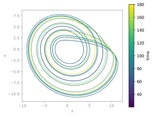
The Rössler orbit projected onto the (x, y) plane, coloured by elapsed time (color_by="time") along a viridis colorbar — the spiral winds outward, then folds. Colour-by-time turns a static orbit into a legible history: you can see which way it is going.

Reading it. The orbit spirals outward in the plane and is periodically folded back inward — the colour ramp (dark → bright with elapsed time) shows the direction of travel, which a bare line cannot. Equal axes keep the spiral round rather than squashed.

---

3-D phase portrait

Three components in space — the attractor itself. Auto-selected for a 3-D trajectory. Hide the axes for a clean "object floating in space" look and frame it with the camera.

lor = ts.systems.Lorenz(ic=[1.0, 1.0, 1.0]).integrate(final_time=100.0, dt=0.01)

(
    lor.to_plot_spec()               # all three → phase_portrait_3d
       .style(axes=False)            # no ticks / labels / grey panes
       .camera(elev=22, azim=-60)    # frame the butterfly
       .save("lorenz-3d.pdf")
)

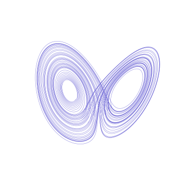
The Lorenz attractor drawn as a 3-D LINE3D portrait. .style(axes=False) strips the ticks, labels, and 3-D background panes; .camera(elev=22, azim=-60) frames the two wings. This is the "attractor floating in space" look the catalogue pages use.

Reading it. The two lobes are the Lorenz butterfly — the orbit loops around one wing, then crosses to the other, never settling. .style(axes=False) is the right choice when the shape is the message and axis numbers add nothing.

Interactive 3-D

A 3-D portrait becomes a rotatable page with the plotly or three.js backend — spec.save("lorenz.html"). See three.js export for the WebGL viewer that ships on the catalogue's 3-D system pages.

---

Spacetime image

A high-dimensional flow — a spatially-extended lattice like Lorenz-96 — imaged as a field: one axis is time, the other is component index, and the state is the colour. Auto-selected when you draw four or more components.

import numpy as np

ic = np.full(20, 8.0)
ic[0] += 0.01                        # a small bump breaks the symmetry
l96 = ts.systems.Lorenz96().integrate(final_time=30.0, dt=0.05, ic=ic)

l96.to_plot_spec().save("lorenz96-spacetime.pdf")   # 20 components → SPACETIME

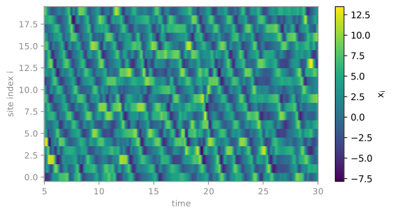
The 20-site Lorenz-96 lattice as a SPACETIME image — time horizontal, site index vertical, state in viridis. The diagonal stripes are travelling waves circulating around the ring of sites; the small initial bump has spread into full spatiotemporal chaos.

Reading it. Each column is the whole lattice state at one instant; scanning left to right plays time forward. The diagonal bands are travelling waves propagating around the periodic ring of sites — the field grows a colorbar and an inferred colour range automatically. transpose=True swaps the two axes if you prefer time on the vertical.

---

Delay embedding

Reconstruct the attractor of a single scalar observable by plotting it against a delayed copy of itself — x(t) vs x(t − τ). This is the natural 2-D view of a delay system, where the true state lives in an infinite-dimensional history space you cannot plot directly.

import numpy as np

mg = ts.systems.MackeyGlass()
traj = mg.integrate(final_time=500.0, dt=0.5,
                    history=lambda s: [1.0 + 0.1 * np.sin(0.2 * s)])

traj.to_plot_spec(kind="delay", tau=17.0).save("mackey-glass-delay.pdf")

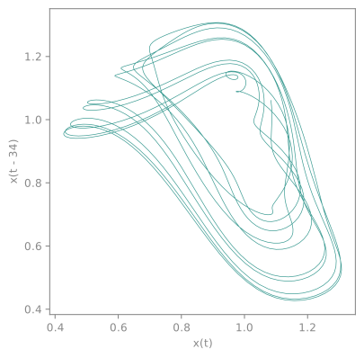
The Mackey–Glass delay system embedded via kind="delay", tau=17.0. At dt=0.5 the delay of 17 time units is a 34-sample lag (the axis reads x(t - 34)), and the folded band is the attractor of the scalar x(t) reconstructed by Takens' theorem.

tau is in time units. It is converted to a sample lag through the trajectory's dt (here 17.0 / 0.5 = 34 samples), so the same tau reads the same physical delay regardless of your output spacing. kind="delay" embeds one component — with no components= it uses the first; select exactly one channel otherwise. See the embedding analysis for choosing an optimal delay from data.

---

Spatial field

The field of a spatially-extended system (a method-of-lines PDE) drawn on its spatial grid — a 1-D profile as a line, a 2-D field as a heatmap. Use kind="field"; the spatial layout comes from the system's _field_shape, so you never pass a shape by hand.

# a 2-D reaction–diffusion field → heatmap of the activator
gs = ts.systems.GrayScott().integrate(final_time=2000.0, dt=5.0)
gs.to_plot_spec(kind="field").save("gray-scott.pdf")           # last field, imshow
gs.to_plot_spec(kind="field", components="v").save("gs-v.pdf")  # pick a field block

A multi-block field (Gray–Scott packs an activator u and inhibitor v) declares field_labels; components= picks the block, defaulting to the last (the activator). A system with no _field_shape (or a 1-D one) plots as a 1-D profile — honest, never guessing a 2-D grid.

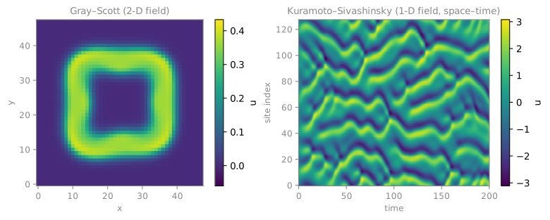
Left: the Gray–Scott activator field via kind="field" — a viridis heatmap of the reaction–diffusion pattern. Right: the Kuramoto–Sivashinsky 1-D field (N=128, L=60) as a space-time diagram (kind="spacetime", viridis) — time horizontal, site index vertical, the chaotic cellular flame front.

A field over time is a movie. to_plot_spec(kind="field", animate=True) plays the field frame by frame — a travelling wave for a 1-D field, an evolving heatmap for a 2-D one. See animation below.

---

Selecting components

components= chooses what to draw — a name, an index, or a sequence — and the auto-dispatch then keys off how many you selected:

traj = ts.systems.Lorenz(ic=[1.0, 1.0, 1.0]).integrate(final_time=100, dt=0.01)

traj.to_plot_spec(components="x")             # one channel  → time series
traj.to_plot_spec(components=["x", "z"])       # two channels → 2-D portrait
traj.to_plot_spec(components=[0, 2])           # …by index, same thing

Names resolve against the system's declared variables (Lorenz's are ('x', 'y', 'z')). A system with no declared names uses generated y0, y1, … labels. An unknown name or an out-of-range index raises InvalidParameterError rather than plotting the wrong thing.

Colour by a scalar

On a time series or a phase portrait, color_by= maps a per-point scalar onto the line — turning a static orbit into a legible history (which way is it going? where is it fast?). It accepts a named field, a per-point array, or a callable f(trajectory) -> array:

traj = ts.systems.Lorenz(ic=[1.0, 1.0, 1.0]).integrate(final_time=100, dt=0.01)

traj.to_plot_spec(components=["x", "z"], color_by="time")     # elapsed time
traj.to_plot_spec(components=["x", "z"], color_by="speed")    # |velocity|
traj.to_plot_spec(components=["x", "z"], color_by=lambda tr: tr["y"])  # any channel

The named fields are computed from the drawn points:

color_by	Meaning
"time"	elapsed time along the orbit
"index"	sample index (0, 1, 2, …)
"speed"	instantaneous speed |dx/dt|
"acceleration" ("accel")	|d²x/dt²|
"arclength"	cumulative distance travelled
"sagitta"	per-point bow (the sampling-error field)
"curvature"	local path curvature

A color_by spec grows a viridis colorbar automatically. Passing color_by to a kind that does not accept it (a spacetime image, say) raises — each per-kind option is valid for one kind only.

Per-kind options

Options that make sense for one kind only ride on **kind_kw rather than cluttering the signature. Passing one to the wrong kind raises InvalidParameterError:

Kind	Option	Meaning
delay	tau (required)	delay in time units (→ sample lag via dt)
time_series, phase_portrait_2d/_3d	color_by	colour the line by a scalar (above)
spacetime	transpose	swap the time / component axes

Rendering and saving

A built PlotSpec renders itself. .save(path) picks the backend from the file extension:

spec = traj.to_plot_spec()

spec.save("fig.pdf")     # vector, for a manuscript  → matplotlib
spec.save("fig.png")     # raster                    → matplotlib
spec.save("fig.svg")     # scalable vector           → matplotlib
spec.save("fig.html")    # interactive, rotatable    → plotly
spec.save("fig.json")    # raw data payload          → json exporter

spec.plot()                       # render inline (a notebook shows it)
spec.render(backend="plotly")     # force a backend

.plot(...) and .save(...) also accept inline tweaks — title=, xlabel=, yscale=, xlim= — applied to the spec before rendering, so a quick one-off needs no chain:

traj.plot(components=["x", "z"], title="Lorenz (x, z)", yscale="linear")

Composing panels

to_plot_spec builds one panel. To arrange several things into one figure — overlaid on shared axes, or tiled — use ts.viz.plot(*things, layout=...), which returns a spec that itself renders:

a = ts.systems.Lorenz(ic=[1.0, 1.0, 1.0]).integrate(final_time=100, dt=0.01)
b = ts.systems.Rossler(ic=[1.0, 1.0, 1.0]).integrate(final_time=200, dt=0.05)

ts.viz.plot(a, b, layout="grid").save("two-attractors.pdf")

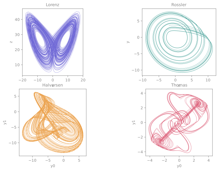
Four attractors tiled into a COMPOSITE grid via ts.viz.plot(lorenz, rossler, halvorsen, thomas, layout="grid") — each its own panel and brand colour. layout= is "overlay" (shared axes), "stack", "row", or "grid".

Overlay merges compatible single-panel specs onto one set of axes, with the legend auto-disambiguated by source:

r1 = ts.systems.Rossler(params={"c": 2.3}, ic=[1.0, 1.0, 1.0]).integrate(400, 0.05).after(100)
r2 = ts.systems.Rossler(params={"c": 5.7}, ic=[1.0, 1.0, 1.0]).integrate(400, 0.05).after(100)

ts.viz.plot(r1, r2, components=["x", "y"], layout="overlay").save("rossler-overlay.pdf")

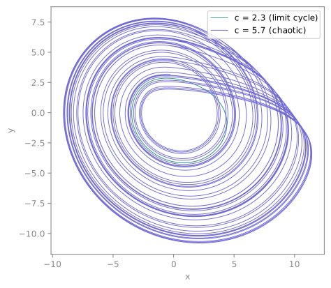
Two Rössler orbits merged onto one (x, y) plane via layout="overlay": the small teal limit cycle (c=2.3) sits inside the wide indigo chaotic band (c=5.7), the legend disambiguated by source. Because plot takes and returns a PlotSpec, a composed figure feeds straight back into another plot call.

Animation

Any spec of any kind becomes a movie by carrying an Animation — an orthogonal modifier, so the semantic kind is unchanged and a backend that cannot animate draws the final frame. Turn it on with animate=True (or a dict / Animation), then tune with the chainable .animate / .trail / .head / .camera / .clock methods:

lor = ts.systems.Lorenz(ic=[1.0, 1.0, 1.0]).integrate(final_time=60.0, dt=0.01)

(
    lor.to_plot_spec(animate=True)
       .animate(n_frames=100, fps=25)
       .trail(("time", 6.0), fade=True)   # a 6-time-unit comet tail, fading
       .head(color="#E8912D")             # an amber "current state" marker
       .style(axes=False)
       .background("#0B0F14")             # a solid dark stage (a GIF has no alpha)
       .save("lorenz-reveal.gif")
)

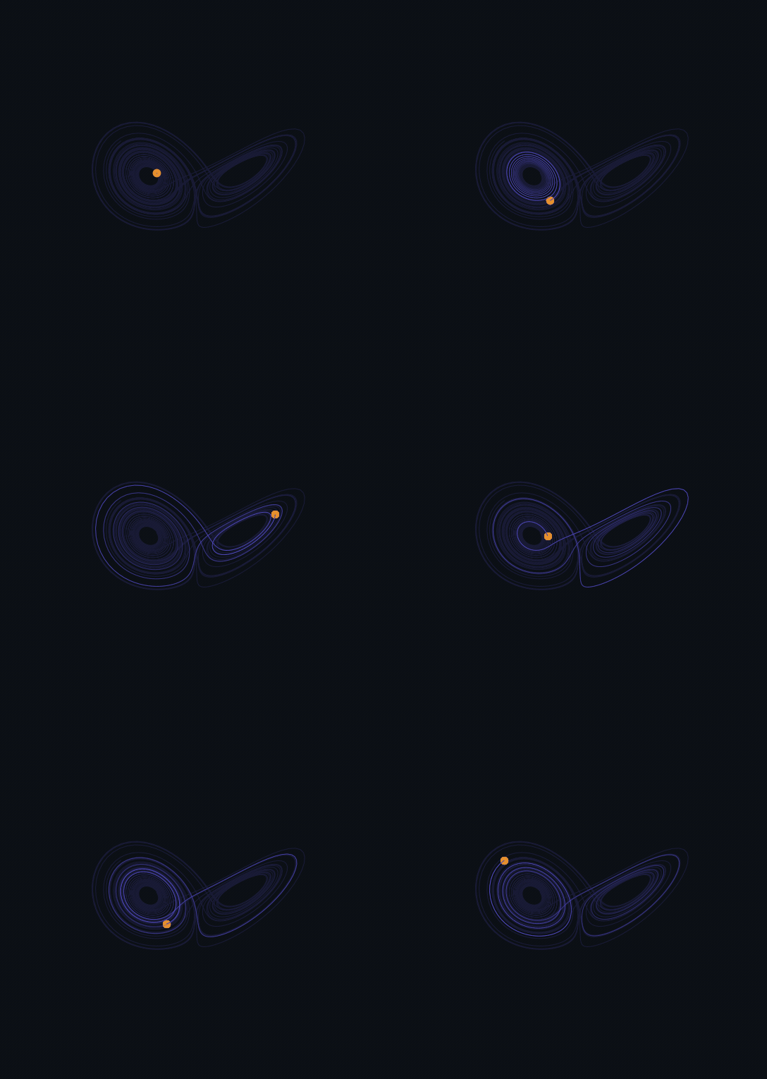
A looping reveal-comet of the Lorenz attractor: animate=True + .trail(("time", 6.0), fade=True) gives a fading 6-time-unit tail behind an amber .head, axes hidden and drawn on the brand dark stage. matplotlib writes .mp4/.gif; plotly exports a real-time rotatable-while-playing .html. See Animation for the field movie, the spinning attractor, and more.

Animate on a solid background

A GIF has no alpha channel — a transparent animation is flattened to one fill colour (often a jarring green). Give a movie a solid background: .background("#0B0F14") here. A still .png/.svg keeps real transparency.

There are two frame models. reveal (the default) keeps the full static data and shows a comet — a head at the current sample, a tail reaching back trail_length (None = a persistent "draws itself in" trail). frames is the spatial-field movie — each frame is a fresh spatial snapshot (used automatically by kind="field", animate=True). Export goes to matplotlib for .mp4/.gif and to plotly for an interactive real-time .html.

Pitfalls

• Random initial conditions. Many catalogue systems have no default IC, so a bare integrate() starts from a fresh random point each run. Always pass an explicit ic= (as every example here does) when you want a figure to reproduce.
• kind="delay" needs tau. It is required, and it is in time units — the trajectory must carry a dt (it does, from integrate) so the lag can be resolved.
• Overlaying incompatible kinds. You cannot overlay an image and a portrait, or a 2-D and a 3-D plot, on one set of axes — use layout="stack" / "grid" to give each its own panel.
• Forcing too few components. kind="phase_portrait_3d" on a 2-D selection raises — pick enough channels, or use "time_series".

See also

• Styling & themes — restyle any spec: colours, widths, themes.
• Figure conventions — the rules for paper-ready output.
• three.js export — interactive WebGL attractor viewers.
• Analysis — every analysis result carries a .plot.