Bogdanov¶

Systems / Maps / Exotic maps

The discrete-time normal form of the Bogdanov-Takens double-zero bifurcation — invariant circles, Arnold tongues, and chaos near a cusp.

discrete · map2 dimensionschaotic

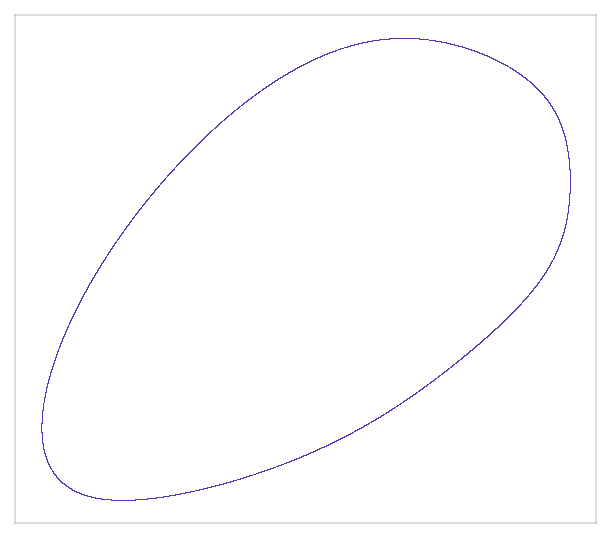
Definition¶

\[ \begin{aligned} y_{0}' &= k y_{0} \left(y_{0} - 1\right) + \mu y_{0} y_{1} + y_{0} + y_{1} \left(eps + 1\right) \\ y_{1}' &= k y_{0} \left(y_{0} - 1\right) + \mu y_{0} y_{1} + y_{1} \left(eps + 1\right) \end{aligned} \]

Parameters¶

Symbol	Default	Role
`eps`	`0`	linear damping/detuning (the Hopf parameter)
`k`	`1.2`	strength of the quadratic x(x-1) nonlinearity
`mu`	`0`	coefficient of the mixed x*y term

Properties¶

Lyapunov spectrum

$+0.001338,\; -0.001338$
computed at build

Kaplan–Yorke dimension

$D_{KY} = 2$

Divergence ∇·f

n/a — discrete map — flow divergence undefined (per-step contraction is |det J|)

Equilibria

2 fixed points
1 stable · 1 unstable

Define it in TSDynamics¶

import tsdynamics as ts

sys = ts.systems.Bogdanov()
traj = sys.iterate(steps=10_000)

exps = sys.lyapunov_spectrum()
ts.kaplan_yorke_dimension(exps)

Reference¶

Bogdanov (1981), Selecta Math. Soviet. 1, 389-421

BibTeX

@misc{bogdanov,
  title = {Bogdanov system},
  note = {Bogdanov (1981), Selecta Math. Soviet. 1, 389-421}
}