Analysis · Attractors & basins

Attractors & basins¶

A Lyapunov exponent or a fractal dimension describes one attractor. But many systems are multistable: several attractors coexist, and which one you reach depends entirely on where you start. That is a global question — it lives in the whole state space, not on a single orbit — and it is the one this toolkit answers. It locates the attractors a system has in a region, paints the basin of initial conditions feeding each, quantifies how tangled the boundaries between them are, tracks how those basins deform as a parameter moves, and measures how robust an attractor is to a perturbation.

Function	Answers	Reads
`find_attractors`	what attractors exist	a system + region
`basins_of_attraction`	which initial condition goes where	a system + `Grid`
`basin_fractions`	each basin's volume share	a system + region
`basin_entropy`	is the boundary fractal?	a label image
`uncertainty_exponent`	boundary dimension $D_0$	a label image
`wada_property`	do ≥ 3 basins share a boundary?	a label image
`continuation`	attractors versus a parameter	a system
`tipping_points`	where a basin dies	a `ContinuationResult`
`resilience`	distance to the boundary	a `BasinsResult`

Everything is built on one engine — a recurrence finite-state machine (Datseris & Wagemakers 2022) — so the same machinery drives maps and flows alike. On a supported engine run (an ODE flow, or a map whose _step lowers) the whole per-initial-condition march runs in one sequential Rust kernel call, bit-identical to the pure-Python fallback.

A bistable example¶

The running example is the damped two-well Duffing oscillator,

\[\ddot{x} = x - x^3 - \delta\,\dot{x},\]

a unit mass in the double-well potential $V(x) = -\tfrac12 x^2 + \tfrac14 x^4$ with linear damping $\delta$. The two wells sit at $x = \pm 1$; with damping, every trajectory eventually rolls into one of them, and which one is exactly the basin question. It is a two-line system:

import numpy as np
import tsdynamics as ts
from tsdynamics import data

class DuffingTwoWell(ts.ContinuousSystem):
    """Damped two-well Duffing: x'' = x - x**3 - delta * x'."""
    params = {"delta": 0.3}
    dim = 2
    variables = ("x", "y")

    @staticmethod
    def _equations(Y, t, *, delta):
        x, y = Y(0), Y(1)
        return (y, x - x**3 - delta * y)

sys = DuffingTwoWell()

# two nearby starts, two different wells:
sys.integrate(final_time=60.0, dt=0.05, ic=[ 1.5, 0.5]).y[-1]   # ≈ [ 1.0, 0.0]
sys.integrate(final_time=60.0, dt=0.05, ic=[-1.5, 0.5]).y[-1]   # ≈ [-1.0, 0.0]

That two stable states coexist is what makes the basin question meaningful. (The delay and stochastic families are not supported here — their state is not a finite-dimensional point the cell tessellation can bin — and raise a clear TypeError.)

Locating attractors¶

find_attractors tessellates a search region into cells, draws random initial conditions from it, and follows each trajectory cell by cell with a small finite-state machine: while it keeps landing in new cells it is transient; once it recurrently re-visits cells it has located an attractor (the recurrent cell set). Near-coincident attractors are proximity-merged (merge_tol).

region = data.Box(np.array([-2.0, -2.0]), np.array([2.0, 2.0]))

att = ts.find_attractors(sys, region, resolution=40, n_seeds=200,
                         dt=0.5, max_steps=2000, seed=0)

att                         # AttractorSet(2 attractors, 0/200 diverged)
[a.center for a in att]     # ≈ [[-1.0, 0.0], [1.0, 0.0]]  — the two well bottoms
att.centers                 # the same, as an (n_attractors, dim) array

Flows step by dt between cell checks, maps by one iteration. A raised or non-finite step is treated as divergence; a finite excursion outside the box is counted by a lost-counter, and a trajectory that never settles within max_steps is reported as diverged. Each Attractor carries its sampled .points, its representative .center, and the number of .cells it occupies.

Tune resolution to the attractor scale

Too coarse and the tessellation merges genuinely distinct attractors; too fine and a chaotic trajectory never recurs into the same cell, so it is never recognised as settled. Size the cells to the attractor's own scale. The per-seed march is sequential by design — earlier seeds leave persistent cell labels that let later seeds settle cheaply, and that shared, order-dependent labelling is exactly what makes the sweep amortise.

Painting basins¶

basins_of_attraction runs that finder from every cell of a Grid of initial conditions and labels each with the attractor it reaches — a colour map of state space. Build the grid with data.Grid(lo, hi, counts) (or the terse data.region([(lo, hi, n), ...])).

grid = data.Grid(np.array([-2.0, -2.0]), np.array([2.0, 2.0]), (60, 60))
basins = ts.basins_of_attraction(sys, grid, dt=0.5, max_steps=2000)

basins.n_attractors        # 2
basins.labels              # int array, one attractor id per cell (−1 = diverged)
basins.labels.shape        # (60, 60)
basins.fractions           # {1: ≈ 0.50, 2: ≈ 0.50}  — basin volume share per id
basins.diverged_fraction   # 0.0  — nothing escaped the box

basins.labels is a plain integer array, ready to plot (attractor id per cell, with -1 marking diverged/unsettled cells). For the two-well Duffing the two basins split the plane roughly in half along the smooth stable manifold of the origin saddle.

Imaging a slice of a higher-dimensional flow

For a flow whose state space is larger than the 2-D picture you want, pass a separate full-dimension recurrence box: the basin is painted over the 2-D Grid of initial conditions while the recurrence FSM runs in the full space (free axes pinned with counts == 1). This is how the magnetic pendulum's famous fractal basins are imaged from its higher-dimensional phase space.

Basin stability¶

basin_fractions skips the image and Monte-Carlo–samples the region instead — basin stability in the sense of Menck et al. (2013): the probability that a random initial condition lands on each attractor, with a binomial standard error $\sqrt{p(1-p)/n}$ that depends only on the fraction and the sample count, never on the dimension.

bf = ts.basin_fractions(sys, region, n=400, dt=0.5, max_steps=2000, seed=0)

bf.fractions        # {1: ≈ 0.53, 2: ≈ 0.47}
bf.dominant         # 1  — the id with the largest basin
bf.standard_error   # {1: ≈ 0.025, 2: ≈ 0.025}
bf.diverged         # 0.0

Because it never forms an image, basin_fractions scales to high dimension where a full grid would be impossible — and it is the workhorse continuation sweeps below.

Validation systems¶

These three examples pin the fractions to values you can check by symmetry:

System	Basins	Each fraction
Two-well Duffing (above)	2	$\approx 1/2$
Newton's method on $z^3 = 1$ (a map)	3 (symmetric)	$\approx 1/3$
Magnetic pendulum	3, fractal boundary	Wada (see below)

Boundary structure¶

Once you have a basin label image — a .labels array — three metrics read it directly and do no further integration, so they run instantly. They answer the question a smooth-boundary two-well system and a fractal-boundary map answer very differently: how predictable is the outcome near the boundary?

For the smooth two-well Duffing basin the answer is "very": the boundary is a clean curve.

be = ts.basin_entropy(basins.labels)
be.sb, be.sbb              # ≈ 0.24, 0.53
be.fractal_boundary        # False   (Sbb ≈ 0.53 < ln 2 ≈ 0.693)

ue = ts.uncertainty_exponent(basins.labels)
ue.alpha                   # ≈ 0.88  — near 1: a thin, nearly-smooth boundary
ue.boundary_dimension      # ≈ 1.12  — D₀ = D − α

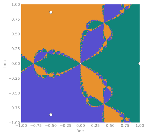
A fractal basin tells a different story. The figure below is Newton's method on $z^3 = 1$ — three roots, three basins, and a Julia-set boundary where every boundary point touches all three colours. That is the Wada property, and wada_property detects it:

from tsdynamics import Grid
from tsdynamics.analysis import basins as bas

class NewtonMap(ts.DiscreteMap):
    """Newton on z**3 - 1 = 0 → three roots, Wada basins."""
    params: dict = {}
    dim = 2
    variables = ("re", "im")
    _jacobian_fd_check = False

    @staticmethod
    def _step(X):
        z = complex(X[0], X[1])
        z = (2.0 * z**3 + 1.0) / (3.0 * z**2)
        return (z.real, z.imag)

    @staticmethod
    def _jacobian(X):
        return ((0.0, 0.0), (0.0, 0.0))

res = bas.basins_of_attraction(
    NewtonMap(), Grid([-1.0, -1.0], [1.0, 1.0], (200, 200)),
    consecutive_recurrences=8, attractor_locate_steps=5, max_steps=200)

res.fractions                    # {1: ≈ 1/3, 2: ≈ 1/3, 3: ≈ 1/3}
wr = ts.wada_property(res.labels)
wr.is_wada, wr.n_basins          # True, 3
wr.fractions[-1]                 # 1.0  — every boundary cell sees all 3 basins

The three basins interleave on a fractal boundary: no matter how finely you localise an initial condition near the boundary, its fate stays uncertain — final-state sensitivity in its purest form.

Fractal Wada basins of the three cube-roots of unity for Newton's map on z^3 = 1 — Basins of Newton's method on $z^3 = 1$: every point in the complex plane is coloured by which of the three roots (the cube roots of unity) it converges to, and the three basins interleave on a fractal Julia-set boundary — the Wada hallmark, where every boundary point touches all three colours.

The three metrics, in one place:

basin_entropyuncertainty_exponentwada_property

The basin entropy $S_b$ and boundary basin entropy $S_{bb}$ (Daza et al. 2016) measure label diversity per box; $S_{bb} > \ln 2$ is a sufficient condition for a fractal boundary, exposed as .fractal_boundary.

import numpy as np
rng = np.random.default_rng(0)
riddled = rng.integers(1, 4, size=(200, 200))   # a maximally-mixed boundary

be = ts.basin_entropy(riddled)
be.sb, be.sbb              # ≈ 1.06, 1.06
be.fractal_boundary        # True   (Sbb > ln 2)

The fraction of $\varepsilon$-uncertain cells scales as $f(\varepsilon)\sim\varepsilon^{\alpha}$ (Grebogi et al. 1983); a small $\alpha$ means a thick, fractal boundary where the outcome is rarely predictable, and the boundary box-counting dimension is $D_0 = D - \alpha$.

ue = ts.uncertainty_exponent(res.labels)   # the Newton basin image
ue.alpha                   # small → fractal, final-state-sensitive boundary
ue.boundary_dimension      # D₀ = D − α

The grid test of Daza et al. (2015) for the Wada property: with three or more basins, a boundary cell is Wada-complete when its neighbourhood contains every basin colour, and the fraction of such cells tends to one for a genuine Wada boundary. A sufficient grid criterion, not a topological proof.

wr = ts.wada_property(res.labels)
wr.is_wada, wr.n_basins        # True, 3   (for the Newton map)

Continuation, tipping, resilience¶

Multistability is not static — as a parameter drifts, basins grow, shrink, and sometimes vanish outright. continuation re-finds the attractors at each value of a swept parameter and matches them across values by state-space distance (greedy nearest; Datseris, Rossi & Wagemakers 2023), so a single attractor keeps its id along its branch. min_fraction drops the tiny spurious sets the recurrence finder can report near unstable equilibria.

Tilt the two-well Duffing with a constant force $F$ — as $F$ grows past a fold, the shallower well disappears, and one basin annihilates:

class TiltedDuffing(ts.ContinuousSystem):
    """x'' = x - x**3 - delta * x' + F  — a fold as F grows."""
    params = {"delta": 0.3, "F": 0.0}
    dim = 2
    variables = ("x", "y")

    @staticmethod
    def _equations(Y, t, *, delta, F):
        x, y = Y(0), Y(1)
        return (y, x - x**3 - delta * y + F)

cont = ts.continuation(TiltedDuffing(), "F", np.linspace(0.0, 0.6, 13),
                       region, n=300, resolution=60, dt=0.5, max_steps=1500, seed=0)

cont.fractions        # {1: [0.52, 0.45, …, nan, nan], 2: [0.48, 0.55, …, 1.0]}
                      #   attractor 1 vanishes past the fold → nan (basin gone)
tips = ts.tipping_points(cont)
[(e["kind"], e["attractor"], round(e["value"], 2)) for e in tips]
# → [("disappear", 1, 0.4)]   — one well's basin annihilates at F ≈ 0.4

tipping_points reads off the parameter values where a basin's share crosses a threshold (default $0$ — true appearance / annihilation); raise the threshold to flag basins shrinking past a safety margin. Each event is a dict with "value", "attractor", "kind" ("appear" / "disappear"), and the "before" / "after" fractions.

resilience measures, for a chosen attractor in a painted BasinsResult, the distance from the attractor to the nearest cell of another basin — the largest perturbation it can absorb without tipping (Halekotte & Feudel 2020):

r = ts.resilience(basins, attractor_id=1)   # from the two-well basin image
float(r)                                     # ≈ 0.61  — distance to the boundary

Larger means more resilient. A resilient attractor sits deep inside its own basin; one hugging the boundary can be tipped by a small kick.

References¶

C. Grebogi, S. W. McDonald, E. Ott and J. A. Yorke, "Final state sensitivity: an obstruction to predictability", Phys. Lett. A 99, 415 (1983).
P. J. Menck, J. Heitzig, N. Marwan and J. Kurths, "How basin stability complements the linear-stability paradigm", Nat. Phys. 9, 89 (2013).
A. Daza, A. Wagemakers, M. A. F. Sanjuán and J. A. Yorke, "Testing for basins of Wada", Sci. Rep. 5, 16579 (2015).
A. Daza, A. Wagemakers, B. Georgeot, D. Guéry-Odelin and M. A. F. Sanjuán, "Basin entropy: a new tool to analyze uncertainty in dynamical systems", Sci. Rep. 6, 31416 (2016).
L. Halekotte and U. Feudel, "Minimal fatal shocks in multistable complex networks", Sci. Rep. 10, 11783 (2020).
G. Datseris and A. Wagemakers, "Effortless estimation of basins of attraction", Chaos 32, 023104 (2022).
G. Datseris, K. L. Rossi and A. Wagemakers, "Framework for global stability analysis of dynamical systems", Chaos 33, 073151 (2023).

System	Basins	Each fraction
Two-well Duffing (above)	2	\(\approx 1/2\)
Newton's method on \(z^3 = 1\) (a map)	3 (symmetric)	\(\approx 1/3\)
Magnetic pendulum	3, fractal boundary	Wada (see below)