Analysis · Fractal dimensions

Fractal dimensions¶

How many directions does an attractor genuinely fill? A strange attractor is not a smooth manifold — it folds a bounded volume onto a set with detailed structure at every scale, and the honest way to count its degrees of freedom is a non-integer dimension. TSDynamics estimates the whole family — the correlation dimension \(D_2\), the generalized Rényi spectrum \(D_q\) (with the capacity \(D_0\) and information \(D_1\) as named cases), and a fixed-mass variant robust into the sparse tails — each fit on a power-law scaling region the library selects automatically and lets you inspect.

Every estimator reads a Trajectory, a raw (N, dim) array, or a 1-D series interchangeably, and returns a DimensionResult that behaves as the dimension number in arithmetic (float(result)) while carrying the log–log curve and the fitted window.

Function	Estimates	Method
`correlation_dimension`	\(D_2\)	Grassberger–Procaccia correlation sum
`box_counting_dimension`	\(D_0\)	box counting (\(q=0\), capacity)
`information_dimension`	\(D_1\)	box counting (\(q=1\), entropy)
`generalized_dimension`	\(D_q\)	box counting, any Rényi order
`dimension_spectrum`	\(D_q\) vs \(q\)	sweeps \(q\) on one partition
`fixed_mass_dimension`	\(D\)	nearest-neighbour (fixed mass)

Correlation dimension¶

The Grassberger–Procaccia correlation sum counts the fraction of point pairs closer than a radius \(r\),

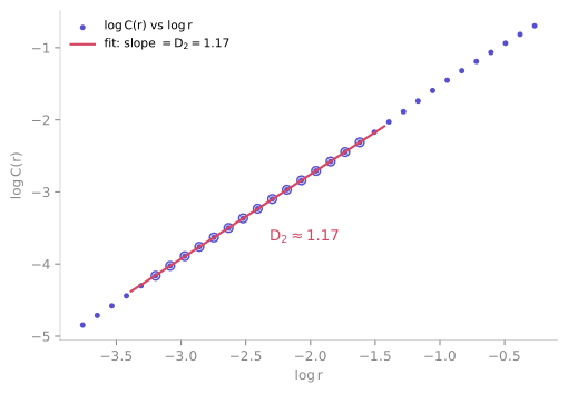
\[ C(r) = \frac{2}{N_\text{pairs}} \sum_{i<j} \Theta\!\big(r - \lVert x_i - x_j \rVert\big), \]

and on a fractal it scales as \(C(r) \sim r^{D_2}\). The correlation dimension is therefore the slope of \(\log C(r)\) against \(\log r\) — but only across the scaling region, the straight middle of the curve. It bends away below (the finite-sampling noise floor) and above (saturation at the attractor diameter), so the slope must be read off the linear stretch, not the whole range.

correlation_dimension computes the sum, then reads \(D_2\) off the automatically selected scaling region. On the Hénon attractor:

import tsdynamics as ts

pts = ts.systems.Henon().iterate(steps=8000, ic=[0.1, 0.1]).y[500:]

res = ts.correlation_dimension(pts, n_radii=32, min_window=8)
float(res)        # 1.171   (the fitted slope D2)
res.stderr        # 0.002   (slope uncertainty over the window)
res.fit_slice     # (3, 13) inclusive indices of the fitted region

The .y[500:] slice drops the transient before the orbit lands on the attractor. The figure plots exactly this result: every point of the log–log curve (indigo), the fitted region circled, and the slope \(D_2\) drawn as the line.

Correlation-dimension scaling of the Hénon attractor — FIG 1 · the Grassberger–Procaccia correlation sum of the Hénon attractor on log–log axes; the slope of the straight scaling region (between the small-r noise floor and the large-r saturation knee) is D₂ ≈ 1.17.

The Theiler window. Temporally adjacent samples of a densely sampled flow sit spuriously close in state space and inflate \(C(r)\) at small \(r\), biasing \(D_2\) downward. Pass theiler=w to count only pairs separated by more than \(w\) samples in time (Theiler 1986) — always set it for a measured flow. The Hénon map above is already decorrelated iterate-to-iterate, so no window is needed; for a reconstructed flow use a few autocorrelation times.

The raw curve is available on its own via correlation_sum(pts), which returns (radii, C) if you want to fit it yourself.

Sanity checks you can run in two lines

A curve of points returns \(D \approx 1\); a filled 2-D region returns \(D \approx 2\). Both are good fixtures for a new pipeline:

import numpy as np
t = np.linspace(0, 2 * np.pi, 4000, endpoint=False)
circle = np.column_stack([np.cos(t), np.sin(t)])
float(ts.correlation_dimension(circle))        # 1.022

square = np.random.default_rng(0).random((5000, 2))
float(ts.correlation_dimension(square))        # 1.906

The generalized spectrum¶

The Rényi (generalized) dimensions partition state space into boxes of side \(\epsilon\) and weight each occupied box by its probability \(p_i(\epsilon)\) raised to a power \(q\) (Hentschel & Procaccia 1983):

\[ D_q = \frac{1}{q-1}\,\lim_{\epsilon \to 0} \frac{\log \sum_i p_i(\epsilon)^q}{\log \epsilon}, \qquad D_1 = \lim_{\epsilon \to 0} \frac{\sum_i p_i \log p_i}{\log \epsilon}. \]

The order \(q\) tunes which part of the measure dominates: \(q=0\) counts every occupied box equally (the capacity, or box-counting, dimension \(D_0\)); \(q=1\) is the information dimension \(D_1\), weighted by the Shannon entropy of the measure; \(q=2\) is the correlation dimension again. For a uniform (monofractal) measure the spectrum is flat; a \(D_q\) that decreases with \(q\) is the signature of multifractality — the attractor's measure is spread unevenly.

pts = ts.systems.Henon().iterate(steps=8000, ic=[0.1, 0.1]).y[500:]

ts.box_counting_dimension(pts)         # D0 = 1.279  (capacity)
ts.information_dimension(pts)          # D1 = 1.230  (entropy)
ts.generalized_dimension(pts, q=2.0)   # D2 = 1.167
ts.generalized_dimension(pts, q=1.5)   # D_1.5 = 1.208  (any real q >= 0)

box_counting_dimension and information_dimension are thin wrappers over generalized_dimension at \(q=0\) and \(q=1\). Negative orders are rejected: the box-counting partition function is dominated by rarely-visited boxes there and becomes unreliable — reach for fixed_mass_dimension if you need the sparse-tail regime.

To read the whole spectrum at once, dimension_spectrum computes the box occupancies once per scale and reuses them across every \(q\), so the full curve costs barely more than a single \(D_q\):

spec = ts.dimension_spectrum(pts, qs=[0, 1, 2, 3, 4])
{q: round(float(r), 3) for q, r in spec.items()}
# {0.0: 1.279, 1.0: 1.230, 2.0: 1.167, 3.0: 1.099, 4.0: 1.141}

It returns a plain dict[float, DimensionResult]. In theory \(D_q\) is non-increasing in \(q\) (\(D_0 \ge D_1 \ge D_2 \ge \dots\)), and that descending trend is the multifractal fingerprint. On a finite sample the leading orders here fall cleanly (\(1.279 \to 1.230 \to 1.167 \to 1.099\)), but the estimate at large \(q\) is noisier — the partition function is then dominated by the most-populated boxes and the fitted slope can wobble slightly (the \(q=4\) value ticks back up to \(1.141\)), so read the low-\(q\) end as the reliable part of the spectrum.

Grid-origin debiasing is automatic

A box count at a single fixed grid origin is biased by where the box boundaries happen to fall: a cluster straddling a boundary is split across two boxes and inflates the count. For every scale, generalized_dimension sweeps several grid-origin offsets and keeps the one yielding the fewest occupied boxes — the minimal cover closest to the true covering number \(N(\epsilon)\). This flattens the \(D_q\) spectrum of a self-similar monofractal (e.g. the middle-thirds Cantor set, \(D_q = \log 2/\log 3\) for all \(q\)). Pass offsets=(0.0,) to recover the naive single-origin partition.

Fixed-mass — robust into the tails¶

The correlation sum fixes a radius and counts the enclosed mass. The fixed-mass method inverts the question: it fixes the mass — the neighbour count \(k\) — and measures the radius \(r_k\) needed to enclose it (Badii & Politi 1985; Grassberger 1985). On a fractal \(k/N \sim r_k^{D}\), so averaging over reference points,

\[ \langle \log r_k \rangle \approx \frac{1}{D}\,\psi(k) + \text{const}, \]

and \(D\) is the slope of the digamma \(\psi(k)\) against \(\langle\log r_k\rangle\). (The digamma — not \(\log k\) — is the bias-free abscissa: for a fixed mass the enclosing radius is a random order statistic, and the digamma correction removes the \(O(1/k)\) bias \(\log k\) carries at small \(k\).)

ts.fixed_mass_dimension(pts)           # 1.266   (agrees with D2)

Because it adapts the radius to the local density, the fixed-mass estimator keeps a usable signal-to-noise ratio deep into the sparse tails of an attractor, where a fixed-radius correlation sum simply runs out of pairs. It is the estimator of choice for higher-dimensional attractors.

Inspect and override the fit¶

Every estimator picks the linear region of its log–log curve automatically, but the number is only as good as that region. The DimensionResult carries the full curve and the chosen window, and two helpers in tsdynamics.analysis.dimensions let you audit or refit it:

from tsdynamics.analysis.dimensions import local_slopes, fit_scaling_region

res = ts.correlation_dimension(pts, n_radii=32, min_window=8)
res.x, res.y            # log r , log C(r)  — the scaling curve
res.fit_slice           # (lo, hi) indices the dimension was fit over

local_slopes(res.x, res.y)      # point-wise slope: a plateau ⇒ scaling
fit = fit_scaling_region(res.x, res.y, min_window=6, tol=1.2)
fit.slope, fit.lo, fit.hi, fit.stderr   # a ScalingFit over the plateau

local_slopes returns the running derivative of the curve; a genuine fractal shows a plateau between the noise floor (small \(r\)) and the saturation knee (large \(r\)), and its height is the dimension. fit_scaling_region scans every contiguous window, keeps those whose straight-line residual is within tol of the best, and returns the widest one — a long clean stretch preferred over a short near-perfect one (Theiler 1990). Tighten tol or raise min_window when the automatic region drifts into a curved tail.

Finite data limits the answer

A reliable \(D\) wants roughly \(10^{D}\) points and a clean plateau spanning at least a decade in scale. Above \(D \approx 5\) prefer fixed_mass_dimension, and never trust a number without looking at local_slopes(res.x, res.y) first — the automatic fit can be fooled by a short spurious flat.

Known values¶

Set	Estimator	Value	Source
Hénon attractor	`correlation_dimension`	\(D_2 \approx 1.17\)	run above
Hénon attractor	`box_counting_dimension`	\(D_0 \approx 1.28\)	run above
Hénon attractor	`fixed_mass_dimension`	\(D \approx 1.27\)	run above
Lorenz attractor	\(D_2\)	\(\approx 2.05\)	literature (Grassberger & Procaccia 1983)
Circle of points	any	\(D \approx 1\)	sanity check
Filled square	any	\(D \approx 2\)	sanity check

Lorenz is a flow — reconstruct first

The Lorenz \(D_2 \approx 2.05\) is a literature value: integrating a flow long enough to populate its attractor densely is slow, so it is cited rather than run inline. In practice you reconstruct the cloud from one observable via delay embedding, then call correlation_dimension on the reconstruction — a full observable-to-dimension pipeline recovers \(D_2 \approx 1.9\) for the (three-dimensional) Rössler attractor.

References¶

P. Grassberger and I. Procaccia, "Characterization of strange attractors", Phys. Rev. Lett. 50, 346 (1983).
H. G. E. Hentschel and I. Procaccia, "The infinite number of generalized dimensions of fractals and strange attractors", Physica D 8, 435 (1983).
R. Badii and A. Politi, "Statistical description of chaotic attractors: The dimension function", J. Stat. Phys. 40, 725 (1985).
P. Grassberger, "Generalizations of the Hausdorff dimension of fractal measures", Phys. Lett. A 107, 101 (1985).
J. Theiler, "Spurious dimension from correlation algorithms applied to limited time-series data", Phys. Rev. A 34, 2427 (1986).
J. Theiler, "Estimating fractal dimension", J. Opt. Soc. Am. A 7, 1055 (1990).