Analysis · Fixed points & periodic orbits
Fixed points & periodic orbits
Every attractor, every bifurcation, every route to chaos is organised by a skeleton of invariant sets — the equilibria a flow can rest at, the fixed points a map holds, the periodic orbits both can loop on. Find that skeleton and you understand the phase portrait: the stable pieces are what you observe, the unstable ones are the saddles that route trajectories between them. This page locates all of them, for maps and flows, each returned with its linear-stability data.
| Function | Finds | For |
|---|---|---|
fixed_points |
\(f(x) = x\) / \(f(x) = 0\) | maps + flows |
periodic_orbits |
period-\(p\) cycles | maps |
periodic_orbit |
a limit cycle | flows |
estimate_period |
dominant period | any signal |
Fixed points and equilibria
A map fixed point solves \(f(x) = x\); a flow equilibrium solves
\(f(x) = 0\) on the right-hand side. fixed_points finds both by multi-start root
finding on the exact analytic Jacobian and classifies each solution from the
Jacobian spectrum, using the right convention for the family — a map fixed point
is stable iff every multiplier \(|\lambda_i| < 1\), a flow equilibrium iff every
eigenvalue has \(\operatorname{Re}\lambda_i < 0\).
import tsdynamics as ts

ts.analysis.fixed_points(ts.systems.Henon())
# [FixedPoint([-1.131354 -0.339406], unstable, |λ|max=3.2598),
#  FixedPoint([0.631354 0.189406], unstable, |λ|max=1.9237)]

ts.analysis.fixed_points(ts.systems.Lorenz())   # the origin and the two C± equilibria
# [FixedPoint([-8.485281 -8.485281 27.], unstable, Re(λ)max=+0.0940),
#  FixedPoint([0. 0. 0.], unstable, Re(λ)max=+11.8277),   # the origin (±0 signs vary)
#  FixedPoint([ 8.485281  8.485281 27.], unstable, Re(λ)max=+0.0940)]
The FixedPoint.continuous flag records which convention was applied and
switches the repr gauge (|λ|max for a map, Re(λ)max for a flow). The
result is a list-like FixedPointSet with .stable / .unstable sublists and
an .eigenvalue_plane() spectrum plot; each FixedPoint carries .x,
.eigenvalues, .stable, and the .plot result surface.
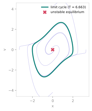
fixed_points) and onto the isolated limit cycle (teal, T ≈ 6.663, from periodic_orbit by single shooting).How it works
- Seeding —
n_seedsrandom points are drawn from a searchregion(default: a burn-in orbit's bounding box padded by 50 %), plus a subsample of a short orbit, biasing the search toward where the dynamics actually live. - Root finding — each seed runs Newton on the residual using the exact analytic Jacobian.
- Dedup & classify — converged roots closer than
dedup_tolare merged, and each survivor is classified from \(J(x^\*)\).
For a flow the equilibria are often off the attractor — the Lorenz origin and
the two \(C^\pm\) centres sit outside the chaotic hull the orbit visits — so when
region is the automatic burn-in box it seeds the search but does not clip the
results, and genuine off-attractor equilibria are kept.
Reaching unstable points: Schmelcher–Diakonos / Davidchack–Lai
Plain Newton has no bias toward stability, but its basin can still miss a
strongly unstable fixed point. For maps, method="sd" / "dl" engage
stabilising transformations that turn an unstable fixed point into a
contracting one, so it can be reached by iteration. Both cycle a set of
orthogonal \(\{-1, 0, 1\}\) matrices \(C\) (one \(\pm 1\) per row and column — \(2^d\,d!\)
of them); for each, the Davidchack–Lai step
is a Newton step regularised by \(\beta\lVert g\rVert\,C^{\mathsf T}\): it reduces
to plain Newton as \(\beta \to 0\) and recovers Newton's quadratic rate near the
root (the regulariser self-anneals). Schmelcher–Diakonos (method="sd") is the
explicit step \(x_{k+1} = x_k + \lambda\,C\,g(x_k)\).
# at r = 4 both logistic fixed points {0, 0.75} are unstable; DL still reaches them
ts.analysis.fixed_points(ts.systems.Logistic(params={"r": 4.0}),
                region=[(-0.2, 1.2)], method="dl")
# [FixedPoint([-0.], unstable, |λ|max=4.0000),
#  FixedPoint([ 0.75], unstable, |λ|max=2.0000)]
Rigorous enumeration: method="interval"
Any multi-start method can silently miss a root whose basin no seed landed in.
method="interval" removes that risk. The Krawczyk operator brackets every
root inside the (required) region by interval branch-and-prune, certifying
existence and uniqueness per sub-box — so the returned set is provably
complete (up to floating-point round-off), it needs no seed, and it is often
faster than multi-start on the analytic systems it applies to. It works for maps
and flows:
# all 27 equilibria of the Thomas system, rigorously, in one box
ts.analysis.fixed_points(ts.systems.Thomas(),
                region=[(-6, 6), (-6, 6), (-6, 6)], method="interval")
# → 27 equilibria  (where a 200-seed Newton finds only 23)
The interval residual and Jacobian are built by forward-mode automatic
differentiation over intervals (an IntervalJet pushed through the map's _step
or the flow's symbolic right-hand side — no symbolic diff), covering
sin/cos/exp/log/sqrt/cosh/tanh/abs and integer powers. A kernel it
cannot enclose — a comparison, a modulo, a non-integer power — raises
InvalidInputError pointing back at method="newton". The arithmetic is
plain-float (rigorous to round-off, machine-precise roots).
Periodic orbits of maps
A period-\(p\) orbit is a fixed point of the \(p\)-fold composition \(f^{p}\), so
periodic_orbits runs the same Davidchack–Lai root finder on
\(g(x) = f^{p}(x) - x\), recovers each orbit by forward iteration, keeps only
orbits of minimal period \(p\) (prime=True drops divisor-period
contaminants — a period-2 orbit is also a fixed point of \(f^4\)), and merges the
cyclic shifts of one orbit.
ts.analysis.periodic_orbits(ts.systems.Logistic(params={"r": 3.2}), 2)
# [PeriodicOrbit(p=2, stable, |μ|max=0.1600, n=2)]

ts.analysis.periodic_orbits(ts.systems.Logistic(params={"r": 3.83}), 3, seed=0)
# [PeriodicOrbit(p=3, unstable, |μ|max=1.6523, n=3),   # the saddle …
#  PeriodicOrbit(p=3, stable,   |μ|max=0.3299, n=3)]   # … and the stable node
The period-3 example is the saddle–node pair born at the tangent bifurcation \(r = 1 + \sqrt{8} \approx 3.8284\) — Davidchack–Lai finds both the stable node and the unstable saddle, where seeding on the attractor alone would reveal only the stable one. Stability of a map orbit is read from the eigenvalues of \(Df^{p}\) at an orbit point (the multipliers), judged against the unit circle.
Periodic orbits of flows (single shooting)
periodic_orbits finds a limit cycle of an autonomous flow by single
shooting: Newton on the unknowns \((x_0, T)\) solving \(\varphi_T(x_0) - x_0 = 0\),
plus an orthogonality phase condition \(f(x_0)\cdot\delta x = 0\) that removes the
trivial time-shift degeneracy. The monodromy matrix
\(M = \mathrm{d}\varphi_T/\mathrm{d}x_0\) comes from integrating the variational
equation alongside the state, and its eigenvalues are the Floquet
multipliers.
class VanDerPolCycle(ts.ContinuousSystem):     # autonomous van der Pol oscillator
    params = {"mu": 1.0}
    variables = ("x", "v")

    def _equations(y, t, mu):
        return [y(1), mu * (1 - y(0) * y(0)) * y(1) - y(0)]

orbits = ts.analysis.periodic_orbits(VanDerPolCycle(params={"mu": 1.0}), 6.0,
                                     ic=[2.0, 0.0], transient=20.0)
print(orbits)
# OrbitSet  1 orbit of period 6 · 1 stable, 0 unstable   (VanDerPolCycle)
#     [0] T = 6.66329  stable  |μ|max = 1  x0 = [ 2.0082 -0.0416]

orbits[0]        # the orbit itself, a (n_points, dim) array
orb = orbits.details[0]
orb.period       # ≈ 6.6633  (the μ = 1 Van der Pol limit-cycle period)
orb.multipliers  # one trivial multiplier ≈ 1 (the flow direction) …
orb.stable       # … and the other inside the unit circle → stable
One verb, one return type. A flow's limit cycle comes back as an OrbitSet
of one, exactly as a map's period-\(p\) orbits do — the second positional argument
is the period: an integer period for a map, a period guess for a flow.
A periodic orbit always carries one trivial Floquet multiplier \(\approx 1\) along
the flow direction; stability is read from the other multipliers. Shooting has
a small basin, so seed it well: transient forward-integrates the guess onto a
stable cycle first (widening the Newton basin), and the guess itself defaults to
an estimate_period read of a burn-in trajectory.
Centres are degenerate
A conservative centre — an undamped harmonic oscillator, for instance — has a
continuum of periodic orbits, so the shooting Jacobian is singular and
Newton collapses onto the equilibrium. periodic_orbit detects the
zero-amplitude collapse (min_amplitude) and raises: shooting needs an
isolated, hyperbolic cycle, not a member of a family.
Estimating a period
Shooting needs a period guess, and often you just want to know a
signal's period. estimate_period reads the dominant period of a sampled signal
— a Trajectory (the sampling step is read from its time grid), a 1-D array, or
a multi-component array (the highest-variance channel by default) — by the first
autocorrelation peak (default) or the dominant spectral frequency:
traj = VanDerPol(params={"mu": 1.0}).run(final_time=300.0, dt=0.01, ic=[2.0, 0.0])
ts.analysis.estimate_period(traj)                  # ≈ 6.66

signal = traj["x"]                        # or any bare 1-D series of your own
ts.analysis.estimate_period(signal, dt=0.01, method="fft")
Both estimators refine the peak parabolically to sub-sample resolution, so a
coarse grid still gives an accurate period. The result is a ScalarResult —
float(result) is the number, and it carries the diagnostic curve for plotting.
The numbers, and the records behind them
Indexing a result set gives you an array, never a class to learn. fps[i] is
the (dim,) point, orbits[i] is the (p, dim) orbit, and np.asarray(...) is
the whole block — so a located root drops straight into arithmetic. The
per-member quantities are vectorised alongside:
fps = ts.analysis.fixed_points(ts.systems.Henon())
fps[0]            # the first root, a (dim,) array
fps.points        # every root, (n, dim)
fps.eigenvalues   # every Jacobian spectrum, (n, dim)
fps.is_stable     # (n,) booleans
The records are one word away, aligned with the same index — reach for them when you want the diagnostics of one member:
fp = ts.analysis.fixed_points(ts.systems.Henon()).details[0]
fp.x, fp.eigenvalues, fp.stable, fp.continuous

orb = ts.analysis.periodic_orbits(ts.systems.Logistic(params={"r": 3.2}), 2).details[0]
orb.points        # the orbit, shape (n_points, dim)
orb.period        # int p (maps) or float T (flows)
orb.multipliers   # eig(Df^p) (maps) or Floquet multipliers (flows)
orb.stable, orb.continuous, orb.residual
FixedPointSet and OrbitSet are list-like CollectionResults: iterate them,
index them, read .stable / .unstable, and call .eigenvalue_plane() to draw
the whole spectrum against its stability boundary (the unit circle for maps, the
imaginary axis for flows).
See also
- Orbit & bifurcation diagrams — where these orbits are born, doubled, and destroyed as a parameter varies
- Poincaré sections — a flow's periodic orbit is a fixed point of its Poincaré map
- Lyapunov spectra — the average stretching rates the multipliers describe locally
- Integration & methods — the RK4 variational core the shooting monodromy rides on
References
- Schmelcher, P. & Diakonos, F. K. (1997). Detecting unstable periodic orbits of chaotic dynamical systems. Phys. Rev. Lett. 78, 4733.
- Davidchack, R. L. & Lai, Y.-C. (1999). Efficient algorithm for detecting unstable periodic orbits in chaotic systems. Phys. Rev. E 60, 6172.
- Krawczyk, R. (1969). Newton-Algorithmen zur Bestimmung von Nullstellen mit Fehlerschranken. Computing 4, 187–201.
- Neumaier, A. (1990). Interval Methods for Systems of Equations. Cambridge University Press.