Tutorial · Anatomy of a chaotic attractor

Anatomy of a chaotic attractor¶

Everyone has seen the Lorenz butterfly. This tutorial takes it apart. We start from three lines of differential equations, integrate them, and draw the attractor — and then we do the thing a picture alone can never do: we certify that the motion is genuinely chaotic and put numbers on it. By the end you will have watched two identical-looking states pull apart, measured the exponential rate at which they do, read the attractor's fractal dimension straight off that measurement, and confirmed it a second, independent way. That chain — integrate, then quantify — is the pattern the whole library is built around.

The example is the Lorenz system (Lorenz, 1963), a three-variable model of thermal convection:

\[ \dot{x} = \sigma(y - x), \qquad \dot{y} = x(\rho - z) - y, \qquad \dot{z} = xy - \beta z, \]

at the classic parameters \(\sigma = 10\), \(\rho = 28\), \(\beta = 8/3\) where its solutions are chaotic.

1. Instantiate the system¶

Lorenz is in the catalogue, so there is nothing to write — just create it. (The next tutorial and the definition guide show how to write your own; the contract is one symbolic _equations method.)

import numpy as np
import tsdynamics as ts

lor = ts.systems.Lorenz()
lor.params       # ParamSet({sigma=10.0, rho=28.0, beta=2.6666666666666665})
lor.variables    # ('x', 'y', 'z')  — named components

Pin the initial condition

The Lorenz class ships with default_ic = None, which means a bare integrate() picks a random start each run. Every snippet below passes an explicit ic=[1.0, 1.0, 1.0] so the printed numbers reproduce exactly. Make this a habit whenever you quote a value: pin the IC (and, for anything stochastic, the seed=).

2. Integrate — and draw the butterfly¶

integrate marches the flow and hands back a Trajectory: a (T, dim) array of states with named components and its provenance in traj.meta.

traj = lor.integrate(final_time=100.0, dt=0.01, ic=[1.0, 1.0, 1.0])

traj.y.shape     # (10001, 3)
traj["z"]        # the z-channel by name
traj.meta["method"]   # the solver that ran — 'rk45'

A three-component trajectory draws as a 3-D phase portrait straight from the front door — to_plot_spec auto-dispatches on the component count. We hide the axes and set a camera angle for a clean "attractor floating in space":

(traj.to_plot_spec()                    # 3 components → PHASE_PORTRAIT_3D
     .style(axes=False)
     .camera(elev=22, azim=-60)
     .save("lorenz.png"))

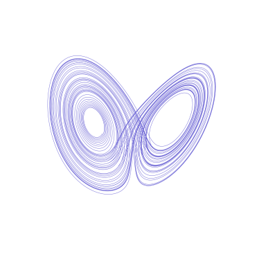
The Lorenz attractor as a 3-D phase portrait with hidden axes — FIG 1 · the Lorenz butterfly — a 3-D phase portrait of the integrated trajectory, axes hidden with `style(axes=False)` and framed with `camera(elev=22, azim=-60)`. Two lobes, a dense fractal weave, and a trajectory that never repeats or self-intersects: the visual signature of a strange attractor.

The picture is suggestive — the trajectory fills a bounded region without ever closing into a cycle — but "looks complicated" is not chaos. For that we need the defining property.

3. The defining property: sensitive dependence¶

Chaos is sensitive dependence on initial conditions: two states that start imperceptibly close separate exponentially fast, so any uncertainty in the present is amplified without limit and long-term prediction becomes impossible — even though the equations are perfectly deterministic. We can watch it directly. Integrate from two initial conditions one part in a billion apart and track the distance between them:

a = ts.systems.Lorenz().integrate(final_time=45.0, dt=0.01, ic=[1.0, 1.0, 1.0])
b = ts.systems.Lorenz().integrate(final_time=45.0, dt=0.01, ic=[1.0 + 1e-9, 1.0, 1.0])

sep = np.linalg.norm(a.y - b.y, axis=1)      # distance vs time
a.t[np.argmax(sep > 1.0)]      # ≈ 34.4  — time for the gap to reach order 1
sep[-1]                        # ≈ 20    — fully decorrelated by t = 45

The two trajectories are visually identical for a while, then the gap explodes: a \(10^{-9}\) initial difference grows to order 1 by \(t \approx 34\) and to the scale of the attractor itself shortly after. That is the predictability horizon — push the starting uncertainty down by another factor of ten and you buy only a constant extra amount of forecast time, because the growth is exponential, not linear. This is the property that makes weather unforecastable weeks ahead no matter how good the measurements.

4. Quantify it: the Lyapunov spectrum¶

Sensitive dependence has a rate, and that rate is the top Lyapunov exponent. The full spectrum \(\lambda_1 \ge \lambda_2 \ge \lambda_3\) gives one number per direction in state space: how fast an infinitesimal ball of nearby states stretches along each axis as it is carried by the flow. lyapunov_spectrum integrates the variational dynamics alongside the state and reads the exponents off a periodically reorthonormalised frame (Benettin et al., 1980):

spec = ts.lyapunov_spectrum(ts.systems.Lorenz(ic=[1.0, 1.0, 1.0]),
                            final_time=300.0, dt=0.05, transient=40.0)

np.asarray(spec)     # ≈ [ 0.903,  0.002, -14.572]
spec.summary()       # "… → chaotic: 1 positive exponent"

Read the signs — they are a fingerprint of the dynamics:

\(\lambda_1 \approx +0.90 > 0\): one expanding direction. A single positive exponent is the working definition of chaos. Its value is the exponential rate we just watched in the separation experiment: \(e^{0.9\,t}\) grows a \(10^{-9}\) gap to order 1 in roughly \(\ln(10^9)/0.9 \approx 23\) time units, the right order of magnitude for the \(t \approx 34\) we measured (the early growth is slower than the asymptotic rate).
\(\lambda_2 \approx 0\): the neutral direction along the flow. Every continuous system has one — perturb a state forward or back along its own trajectory and it neither grows nor shrinks. It lands just above zero numerically rather than exactly on it.
\(\lambda_3 \approx -14.6 < 0\): a strongly contracting direction. This is what pins the motion onto a thin attractor instead of filling space.

That the exponents are positive, zero, negative — in that order — is the signature of a chaotic dissipative flow. There is even an exact check: the sum of the exponents equals the average divergence of the vector field, which for Lorenz is the constant \(-(\sigma + 1 + \beta)\):

float(np.sum(np.asarray(spec)))     # ≈ -13.667
-(10.0 + 1.0 + 8/3)                 #    -13.667  — phase-space volume shrinks at this rate

Perfect agreement: the flow contracts a phase-space volume by a factor \(e^{-13.667}\) per unit time, which is why any blob of initial conditions collapses onto the zero-volume attractor.

Only need the top exponent?

When you just want the leading rate — or the right-hand side is non-smooth and has no analytic Jacobian — max_lyapunov runs the classic two-trajectory method using nothing but the stepping protocol: ts.max_lyapunov(ts.systems.Lorenz(ic=[1.0, 1.0, 1.0]), dt=0.05) returns ≈ 0.89, agreeing with \(\lambda_1\) from the full spectrum.

5. The attractor's dimension — two ways¶

A strange attractor is not a smooth surface: it folds a bounded volume onto a set with structure at every scale, and its honest "size" is a non-integer dimension. The Lyapunov spectrum already contains it. The Kaplan–Yorke dimension interpolates between the expanding and contracting directions — \(D_{KY} = j + (\lambda_1 + \dots + \lambda_j)/|\lambda_{j+1}|\) at the point where the cumulative exponent sum crosses zero (Kaplan & Yorke, 1979):

spec.kaplan_yorke        # ≈ 2.062
ts.kaplan_yorke_dimension([0.903, 0.002, -14.572])   # ≈ 2.062  — the same, from the bare numbers

\(D_{KY} \approx 2.06\): the Lorenz attractor is just more than a two-dimensional surface — a sheet with enough fractal crinkle to nudge it past dimension 2.

Now confirm it independently, without any Jacobian, by measuring the geometry of the point cloud directly. The correlation dimension (Grassberger & Procaccia, 1983) counts how the fraction of close point-pairs scales with radius:

cloud = ts.systems.Lorenz().integrate(final_time=200.0, dt=0.02, ic=[1.0, 1.0, 1.0]).y[2000:]
ts.correlation_dimension(cloud, theiler=200)     # ≈ 2.06

The two numbers agree to two decimal places from completely different routes — one from the dynamics (tangent-space stretching), one from the static geometry (pairwise distances). When a dynamical and a geometric estimate of the attractor's dimension concur, you can trust both. (The theiler=200 window excludes temporally-adjacent samples, which sit spuriously close on a densely sampled flow and would otherwise bias the estimate — always set it for a flow.)

6. Watch it draw itself¶

Finally, for a talk or a paper's supplementary material, the same spec animates: a reveal-comet traces the trajectory as it is integrated, a fading tail behind the moving head.

(traj.to_plot_spec(animate=True)
     .animate(n_frames=120, fps=30)
     .trail(("time", 6.0), fade=True)     # 6-time-unit fading tail
     .head(color="#F5A623")               # amber "current state" dot
     .style(axes=False)
     .camera(elev=22, azim=-60)
     .save("lorenz.gif"))

The .mp4 / .gif extensions render through matplotlib; a .html extension instead exports a real-time interactive Plotly comet you can rotate while it plays. See the visualization section for the full animation model.

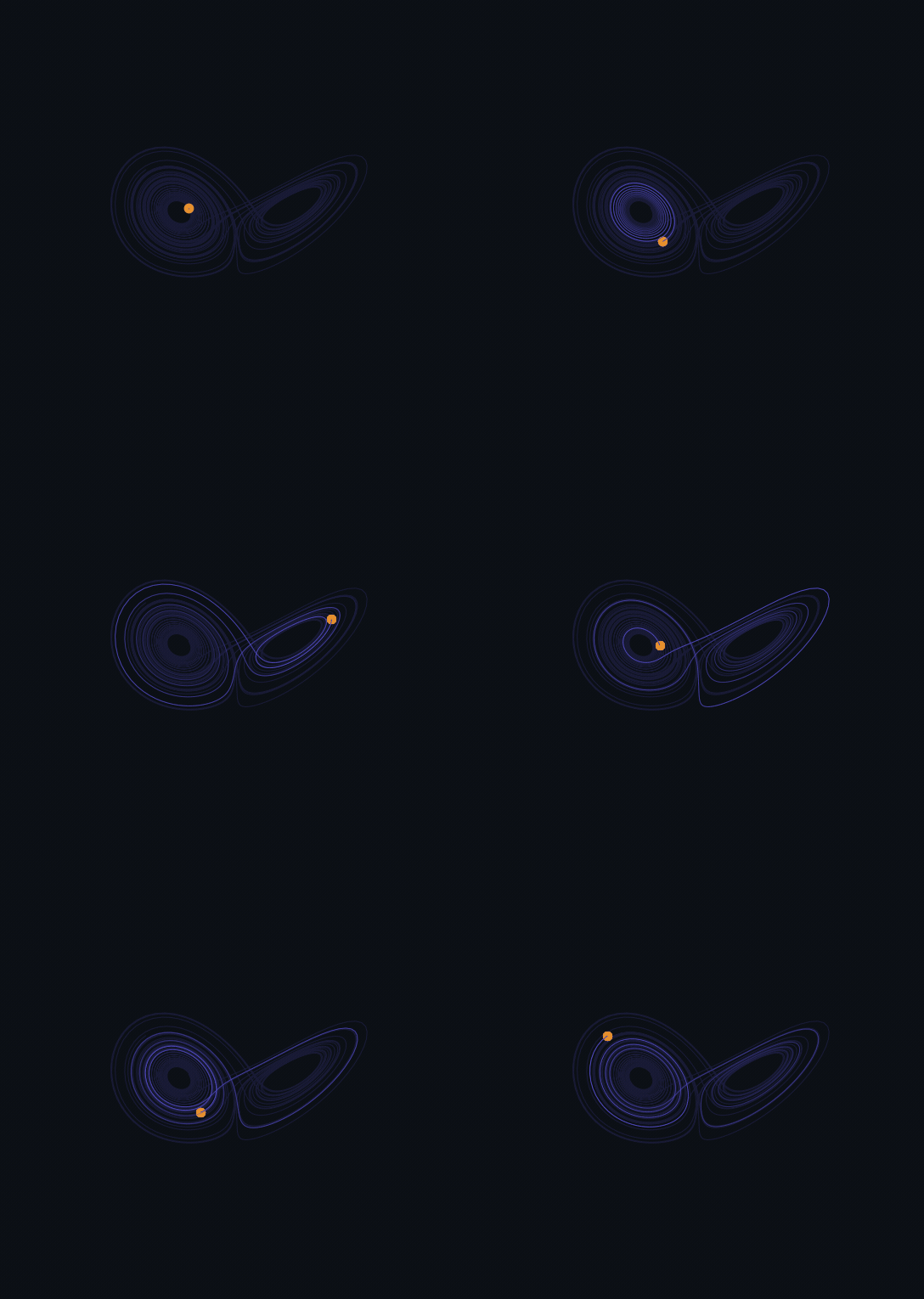
Animated reveal of the Lorenz attractor drawing itself in — FIG 2 · the same trajectory as a looping reveal comet — a fading trail follows the amber current-state marker as the butterfly draws itself in. One `PlotSpec`, one `.save("…gif")`.

What you built¶

From a catalogue system and half a dozen calls you produced the complete chaos certificate: the attractor drawn, sensitive dependence witnessed, the Lyapunov spectrum computed with its signs read, the phase-volume contraction checked against theory, and the fractal dimension pinned down two independent ways. Every result carries its settings in traj.meta / the result's .meta, so the whole thing is reproducible and auditable.

That is the arc the library is built for: define the system once, then compose analysis on top of it. The next tutorial asks the sequel question — where does this chaos come from as a parameter is turned?

References¶

Lorenz, E. N. (1963). Deterministic nonperiodic flow. J. Atmos. Sci. 20, 130–141.
Benettin, G., Galgani, L., Giorgilli, A. & Strelcyn, J.-M. (1980). Lyapunov characteristic exponents for smooth dynamical systems … Meccanica 15, 9 & 21.
Kaplan, J. L. & Yorke, J. A. (1979). Chaotic behavior of multidimensional difference equations. LNM 730, 204.
Grassberger, P. & Procaccia, I. (1983). Measuring the strangeness of strange attractors. Physica D 9, 189–208.