References · Benchmarks

Benchmarks¶

A library is only as good as the numbers it produces and the time it takes to produce them. This page is the honest, reproducible comparison of TSDynamics on the classic integration and analysis tasks — the same tasks run through each library's own code, timed the same way, on the same machine — against two references: the Python ecosystem a user would actually reach for, and DynamicalSystems.jl, the mature compiled-Julia stack that is the fastest thing in the field.

The headline against Python is the integration engine: on the Lorenz system TSDynamics' Rust backend produces the whole dense trajectory ~62× faster than SciPy's solve_ivp with the interpreter, ~134× faster with the JIT, and ~200–450× faster than dysts — at the same accuracy. Against DynamicalSystems.jl the story is different and, for a Python-facing library, telling: on the tasks with substantial work — integration, the embedded correlation dimension — it is within ~2× of Julia and often as accurate or more accurate, tying the reference on the correlation dimension while being ~20× more accurate and pinning the Hénon fixed point to the same machine precision. On the tight map loops where Julia pulls further ahead, both libraries already finish in microseconds to single-digit milliseconds — a gap no workflow feels.

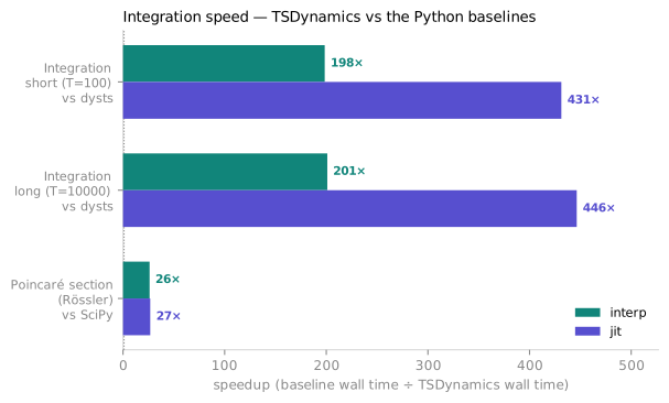
Horizontal bar chart of integration speedups: TSDynamics interp and jit versus SciPy and dysts on the short, long, and Poincaré tasks — Integration is TSDynamics' clear strength over Python. Bars are the recorded best-of-N wall-time ratios: the Rust engine (teal · `interp`, indigo · `jit`) integrates the Lorenz system in one dense call ~62–156× faster than SciPy and ~200–450× faster than dysts, and marches the Rössler Poincaré section ~26× faster than SciPy's event integrator.

Methodology¶

Every number on this page comes from a single full run of the cross-library harness in the repository's benchmarks/ folder. The methodology is designed to be fair to every library and reproducible on any machine.

Best-of-N wall time. Each task is timed \(N\) times and the minimum is kept — the most reproducible estimator of intrinsic cost, since the machine can only ever add noise, never remove it. A warm-up call is made before timing, so one-time compilation (TSDynamics' tape lowering, numba's JIT, Julia's method compilation) is paid once and excluded from the measured time.
The library's own code, each task. The integration tasks each use the library's own integrator — that is the entire point of an integration benchmark. The from-data analysis tasks feed every library the same generated time series (dumped once, independently of any benchmarked library), so the comparison measures the estimator, not the input.
Matched settings across libraries. Where a task has a tunable that changes the work done — the Lyapunov renormalisation interval, the fixed-point search method — TSDynamics is run with the same setting as the reference it is compared against (e.g. the Julia Δt=0.1 renorm step, the same \([-2,2]^2\) box and rigorous method for fixed points), so the comparison is apples-to-apples.
Process isolation. Every library runs in its own subprocess and writes a JSON record the orchestrator merges. A crash, a slow library, or an import side-effect cannot take the rest of the suite down, and each library gets a clean interpreter.
Precision against a tight reference. Where a task has a ground truth — a literature Lyapunov exponent, an analytic fixed point, a \(10^{-13}\) reference trajectory — the table reports both the estimate and its deviation \(\Delta\) from that reference.

The environment¶


Platform	Linux x86-64 (`glibc` 2.43)
Python	3.12.12
TSDynamics	5.2.4 (`interp` + `jit` backends)
DynamicalSystems.jl	3.6.8 (Julia 1.12)
NumPy	`< 2.5` (pinned — numba, and therefore pynamical/nolitsa, does not yet build on NumPy 2.5)

Reproduce it yourself

The harness, adapters, frozen inputs and rendered tables all live under benchmarks/ in the source tree. It runs out of a dedicated virtual-env so it never perturbs the project's own — see benchmarks/README.md for the one-time setup and the run_benchmarks.py invocations. The numbers below are the committed output of one full run; re-running on your own hardware will shift the absolute times but not the relative story.

The libraries compared¶

Each library contributes what it is designed for; a library that does not provide a capability leaves that cell blank.

Library	Version	What it contributes to the comparison
TSDynamics (`interp` + `jit`)	5.2.4	the library under test — every task, both engine backends
DynamicalSystems.jl	3.6.8	the compiled-Julia reference — integration, Lyapunov, bifurcation, Poincaré, fixed points, basins, correlation dimension
SciPy	1.18.0	the integration baseline (`solve_ivp`), fixed points (`fsolve`), Poincaré (events)
dysts	0.96	a chaotic-systems catalogue on a SciPy integrator; correlation dimension (`gp_dim`), DFA
pynamical	0.3.3	the logistic-map bifurcation diagram (numba)
nolds	—	from-data correlation dimension, Rosenstein Lyapunov, sample entropy, DFA, Hurst
nolitsa	—	from-data correlation dimension, MLE Lyapunov, FNN embedding dimension, IAAFT surrogates (numba)
antropy	0.2.2	sample / permutation entropy, DFA
neurokit2	0.2.13	broad from-data complexity — entropy, DFA, Hurst, correlation dim, RQA, embedding dim, surrogates
pyunicorn	0.9.0	recurrence quantification (RQA determinism)

Two further libraries were evaluated but could not be run in this environment, and are recorded here for completeness: PyDSTool (does not import on NumPy ≥ 2 — the removed numpy.distutils) and TISEAN (legacy C/Fortran CLI tools that do not build with the current toolchain).

Integration speed¶

The core task. Integrate the Lorenz system with DOP853 at rtol=atol=1e-9 and return the trajectory. dysts and DynamicalSystems.jl join the integration rows; the from-data-only Python libraries correctly leave these cells blank.

Task	TSDynamics `interp`	TSDynamics `jit`	SciPy	dysts	DynamicalSystems.jl
Integration — short (\(T=100\))	7.78 ms	3.58 ms	480.47 ms	1.544 s	1.72 ms
Integration — long (\(T=10000\))	780.08 ms	351.24 ms	54.921 s	156.802 s	196.03 ms
Poincaré section (Rössler, \(y=0\))	202.93 ms	198.11 ms	5.306 s	—	14.11 ms

Reading the ratios:

vs Python: short integration is 62× (interp) / 134× (jit) faster than SciPy and 198× / 431× faster than dysts; the long run holds the win at 70× / 156× vs SciPy and 201× / 446× vs dysts. The Poincaré section marches the whole attractor and refines every crossing in one call, ~26× faster than SciPy's event-based solve_ivp.
vs Julia: DynamicalSystems.jl is faster — but only by ~2× on both the short and long integrations (jit 3.58 ms vs 1.72 ms; 351 ms vs 196 ms). For a Python-facing library against a decade-tuned compiled-Julia integrator, ~2× is a narrow gap. On the Poincaré section Julia's compiled event handling keeps a wider ~14× edge.

The jit backend (Cranelift) roughly halves the interpreter's time on the raw integration tasks; on the event-driven Poincaré task, where crossing refinement dominates, the two backends are within noise of each other.

Integration accuracy¶

Speed is only half the story. Integrated to \(T=8\) with DOP853 at rtol=atol=1e-10, how close is the final state to a \(10^{-13}\) reference trajectory (itself a SciPy DOP853 run at that tolerance)?

Task	TSDynamics `interp`	TSDynamics `jit`	SciPy	DynamicalSystems.jl
\(\lVert \Delta \rVert_\infty\) vs \(10^{-13}\) reference	\(3.33\times10^{-9}\)	\(3.33\times10^{-9}\)	\(2.83\times10^{-9}\)	\(1.77\times10^{-10}\)
Wall time for that run	299 µs	308 µs	25.64 ms	55 µs

Every adaptive integrator hits the reference trajectory to \(\lesssim 10^{-9}\) at matched tolerance. TSDynamics costs nothing in accuracy for its ~86× speed advantage over SciPy — interp and jit are bit-for-bit identical here. DynamicalSystems.jl lands about an order of magnitude tighter (\(1.8\times10^{-10}\)) in about a fifth of the time; both are far below any practically meaningful error for a chaotic Lorenz trajectory.

Alongside DynamicalSystems.jl¶

DynamicalSystems.jl — a mature stack on Julia's LLVM-compiled DifferentialEquations.jl — is the fastest dynamical-systems software there is, so it is the reference worth measuring against. Fed the same tasks at matched settings, two things are true at once.

Where the work is substantial, TSDynamics is level with it. On the tasks that do enough computation for wall time to mean anything, TSDynamics is within ~2× of Julia — and where they tie on speed, it is more accurate:

Task	TSDynamics	DynamicalSystems.jl
Correlation dimension (embedded)	210.66 ms	202.02 ms	parity — and ~20× more accurate (\(\Delta\,0.004\) vs \(0.079\))
Integration — long (\(T=10000\))	351.24 ms	196.03 ms	~2×, both accurate to \(\ll 10^{-8}\)
Integration — short (\(T=100\))	3.58 ms	1.72 ms	~2×

That a Python library reaches within ~2× of DifferentialEquations.jl on the dense integration — returning the whole trajectory in one FFI call rather than stepping from Python — is the number that matters, and it comes with matching or better accuracy (parity on the correlation dimension, a machine-precision fixed point).

Julia is faster on the remaining analysis routines — the Lyapunov spectrum (78 ms vs 18 ms), basins (58 ms vs 21 ms), the Poincaré section (198 ms vs 14 ms), the from-data Lyapunov (34 ms vs 3 ms). Its compiled variational and event kernels are excellent, and TSDynamics matches it on the answer every time — identical basin labels, the same Poincaré crossings, a \(\Delta < 10^{-3}\) spectrum. Those native loops are exactly where the engine grows next.

On the tight map loops, both are already instant — the ratio is between two tiny numbers. These finish in single-digit milliseconds or microseconds:

Task	TSDynamics	DynamicalSystems.jl
Bifurcation diagram (1000-rate sweep)	6.56 ms	1.15 ms
Max. Lyapunov (Hénon map)	5.56 ms	99 µs
Fixed points (Hénon, box method)	2.37 ms	94 µs

Quoting a "50×" here would be true and useless: 5 ms versus 0.1 ms is not a gap anyone iterates or bifurcates around, and TSDynamics still returns the same answer — the Hénon fixed point to the identical \(1.1\times10^{-16}\) as Julia's rigorous method. Moving these tight map/event loops fully into the Rust engine, as the trajectory path already is, is on the roadmap; we'll put a proper head-to-head here once we are at or past Julia on them.

The analysis toolkit vs Python¶

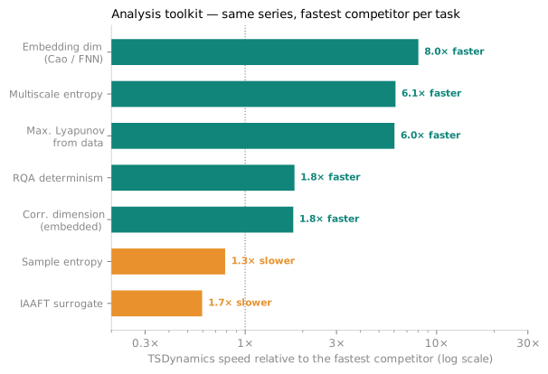
For the from-data analysis routines the harness feeds every library the same generated series, so the comparison isolates the estimator. TSDynamics ranges from competitive to comfortably fastest across most of these — and, honestly, loses three tight inner loops.

Horizontal bar chart on a log axis showing TSDynamics analysis-toolkit speed relative to the fastest competitor per task; wins in teal, losses in amber — Same series, every Python library, fastest competitor per task. Teal bars (to the right of the 1× line) are tasks where TSDynamics is fastest — embedding dimension, correlation dimension, the from-data Lyapunov, RQA and multiscale entropy. Amber bars are the honest losses: the specialised entropy and IAAFT-surrogate estimators edge it out.

Where TSDynamics leads¶

Task	TSDynamics	Best competitor	Speedup
Embedding dimension (Cao / FNN)	26.84 ms	neurokit2 215.65 ms · nolitsa 1.678 s	8.0× / 63×
Correlation dimension (embedded)	210.66 ms	nolitsa 375.71 ms · dysts 1.220 s · nolds 1.864 s	1.8× – 8.8×
Maximal Lyapunov from data	33.68 ms	nolitsa 202.98 ms · nolds 283.17 ms	6.0× / 8.4×
RQA determinism	19.29 ms	pyunicorn 34.91 ms · neurokit2 151.11 ms	1.8× / 7.8×
Multiscale entropy	30.54 ms	neurokit2 186.36 ms	6.1×

Where the other libraries win¶

TSDynamics is not universally fastest, and the benchmark says so plainly:

Task	TSDynamics	Fastest competitor	Verdict
Sample entropy	21.09 ms	neurokit2 16.57 ms · antropy 18.09 ms	~1.3× slower than the specialised C-accelerated estimators (but ~23× faster than nolds' pure Python)
Permutation entropy	211 µs	antropy 87 µs	~2.4× slower than antropy's tight NumPy kernel (but ~11× faster than neurokit2)
IAAFT surrogate	25.01 ms	neurokit2 14.90 ms · nolitsa 21.76 ms	~1.7× slower than the specialised surrogate generators

These are all cheap, tight inner loops where a single-purpose kernel has the edge — and all three land in the tens-of-milliseconds-or-less range, so the absolute cost is small either way.

Precision where there is a ground truth¶

Speed means nothing without the right answer. On every task with a literature or analytic reference, here is the estimate and its deviation \(\Delta\).

Task (reference)	TSDynamics	\(\Delta\)	DynamicalSystems.jl	Notable others
Correlation dimension — Lorenz \(= 2.05\)	2.054	\(3.9\times10^{-3}\)	1.971 (\(\Delta\,0.079\))	nolitsa 2.055 · dysts 2.014 · nolds 1.905
Fixed point — Hénon \(x^* = 0.6314\)	0.6314	\(1.1\times10^{-16}\)	0.6314 (\(\Delta\,1.1\times10^{-16}\))	SciPy 0.6314 (\(\Delta\,2.3\times10^{-14}\))
Maximal Lyapunov — Hénon \(= 0.419\)	0.4231	\(4.1\times10^{-3}\)	0.4222 (\(\Delta\,3.2\times10^{-3}\))	nolitsa 0.4176 · nolds 0.3721
Lyapunov spectrum — Lorenz \(\lambda_{\max} = 0.9056\)	0.9288	\(2.3\times10^{-2}\)	0.9086 (\(\Delta\,3.0\times10^{-3}\))	—
Integration accuracy (Lorenz \(T=8\))	—	\(3.33\times10^{-9}\)	—	SciPy \(2.83\times10^{-9}\) · jl \(1.77\times10^{-10}\)

The takeaways:

TSDynamics is the most accurate on the embedded correlation dimension on this page — closer to the reference than the Julia stack and every Python library — and pins the Hénon fixed point to the same machine precision as Julia's rigorous box method.
On the maximal Lyapunov exponent the two are a statistical tie; on the Lyapunov spectrum at a matched renormalisation step Julia is the more accurate, and the page says so.
Cross-library agreement validates the shared-series tasks. Fed identical input, sample entropy lands at \(\approx 0.143\) and permutation entropy at \(\approx 0.451\) to three digits across TSDynamics, antropy and neurokit2; DFA/Hurst sit at \(\approx 0.5\) on white noise; RQA determinism at \(\approx 0.99\). Agreement is the point — it means every library, including TSDynamics, computes the same quantity the same way.

One honest caveat: from-data Lyapunov¶

The maximal-Lyapunov-from-data task is famously method- and parameter-sensitive, and it is worth calling out because every library misses the literature value:

Method	Estimate (\(\lambda_{\max}\), ref \(= 0.9056\))
TSDynamics (Rosenstein)	1.29
nolitsa (Rosenstein)	1.299
nolds (Rosenstein)	1.24
DynamicalSystems.jl (Kantz)	0.613

On a deliberately oversampled Lorenz series the Rosenstein-family estimators all cluster near \(1.3\), while the Kantz estimator undershoots — the spread is the method and the (hard, oversampled) problem, not a ranking of the libraries. It is exactly the kind of result the from-data Lyapunov page tells you to treat with care: inspect the scaling region before trusting the slope.

What the comparison shows¶

The durable, machine-independent takeaways:

Against Python, integration is a decisive win. The Rust engine is ~62–156× faster than SciPy and ~200–450× faster than dysts, at the same accuracy, returning the whole dense trajectory in one call.
Against DynamicalSystems.jl — the fastest software in the field — TSDynamics is within ~2× on the substantial integration and dimension work and level on accuracy. Parity on the correlation dimension (and more accurate there), ~2× on integration; Julia is faster on the analysis routines, but the largest gaps are on tasks both libraries finish in single-digit milliseconds or microseconds, and TSDynamics returns the same answer. Those native map/event loops are the roadmap's next target.
Precision is excellent wherever there is a ground truth — the most accurate embedded correlation dimension on the page, a machine-precision fixed point matching Julia's rigorous method.
It is not fastest everywhere, and this page says so. Specialised kernels win the tightest inner loops (sample/permutation entropy, IAAFT surrogates), and Julia's compiled map loops win the Hénon Lyapunov and Poincaré tasks — the clear place future engine work would pay off, the honest flip-side of the integration story.