Hopfield

Systems / ODEs / Exotic systems

A six-neuron continuous Hopfield network whose recurrent inhibition drives the neural activity chaotic (Lewis–Glass).

continuous · ODE6 dimensionschaotic

spatiotemporal field

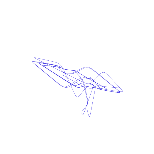
Definition

\[ \begin{aligned} \dot{x1} &= - \beta + \frac{\tanh{\left(eps \left(- x_{2} - x_{5} - x_{6}\right) \right)}}{2} + \frac{1}{2} - \frac{x_{1}}{\tau} \\ \dot{x2} &= - \beta + \frac{\tanh{\left(eps \left(- x_{4} - x_{5} - x_{6}\right) \right)}}{2} + \frac{1}{2} - \frac{x_{2}}{\tau} \\ \dot{x3} &= - \beta + \frac{\tanh{\left(eps \left(- x_{1} - x_{2} - x_{5}\right) \right)}}{2} + \frac{1}{2} - \frac{x_{3}}{\tau} \\ \dot{x4} &= - \beta + \frac{\tanh{\left(eps \left(- x_{1} - x_{2} - x_{3}\right) \right)}}{2} + \frac{1}{2} - \frac{x_{4}}{\tau} \\ \dot{x5} &= - \beta + \frac{\tanh{\left(eps \left(- x_{1} - x_{2} - x_{4}\right) \right)}}{2} + \frac{1}{2} - \frac{x_{5}}{\tau} \\ \dot{x6} &= - \beta + \frac{\tanh{\left(eps \left(- x_{2} - x_{3} - x_{4}\right) \right)}}{2} + \frac{1}{2} - \frac{x_{6}}{\tau} \end{aligned} \]

Parameters

Symbol	Default	Role
beta	0.5	tonic drive
eps	10	synaptic gain
tau	2.5	membrane time constant

State variables: x1, x2, x3, x4, x5, x6

Properties

Lyapunov spectrum

$+0.08992,\; +0.0007919,\; -0.3216,\; -0.3889,\; -0.3669,\; -1.413$
computed at build

Kaplan–Yorke dimension

$D_{KY} = 2.282$

Divergence ∇·f

$\nabla\!\cdot f = - \frac{6}{\tau}$
constant

Equilibria

none found (no equilibria)

Define it in TSDynamics

import tsdynamics as ts

sys = ts.systems.Hopfield()
traj = sys.integrate(final_time=100.0, dt=0.01)

exps = sys.lyapunov_spectrum()
ts.kaplan_yorke_dimension(exps)

Reference

Lewis & Glass (1992), Neural Comput. 4, 621-642

BibTeX

@misc{hopfield,
  title = {Hopfield system},
  note = {Lewis & Glass (1992), Neural Comput. 4, 621-642}
}