Analysis · Delay embeddings

Delay embeddings¶

Most of the analysis toolkit wants a state-space cloud — a point per instant in the system's phase space. But an experiment usually hands you a single scalar channel: a voltage, a concentration, a brightness. Takens' embedding theorem says that is enough. From one generic observable \(x(t)\) of a deterministic system you can reconstruct a trajectory whose attractor is diffeomorphic to the true one — same topology, same invariants (correlation dimension, Lyapunov spectrum) — by stacking time-delayed copies of the single signal into a vector:

\[ y_i = \big(x_i,\; x_{i+\tau},\; x_{i+2\tau},\; \dots,\; x_{i+(m-1)\tau}\big). \]

Takens (1981) guarantees this delay-coordinate map is an embedding for a generic observable once \(m > 2d\), where \(d\) is the box-counting dimension of the original attractor. Two choices make the reconstruction good in practice — the delay \(\tau\) and the dimension \(m\) — and TSDynamics provides a principled heuristic for each. All three functions live under tsdynamics.analysis.embedding and are re-exported at the top level:

import tsdynamics as ts
from tsdynamics.analysis.embedding import (
    embed, optimal_delay, mutual_information, autocorrelation,
    embedding_dimension, cao_dimension, false_nearest_neighbors,
)

The reconstruction, from one channel¶

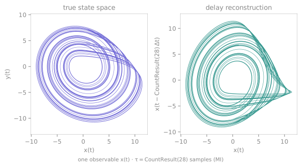
The figure makes the theorem concrete. On the left is the true \((x, y)\) projection of the Rössler attractor; on the right is a delay reconstruction built from the single observable \(x(t)\) — the \(y\) channel is never used, yet the reconstructed loop is topologically the same object.

ros = ts.systems.Rossler()
traj = ros.integrate(final_time=400.0, dt=0.05, ic=[1.0, 0.0, 0.0])
x = traj.y[1000:, 0]        # keep ONLY the x channel

tau = ts.optimal_delay(x, method="mi", max_delay=120)   # 27 samples
emb = ts.embed(x, dimension=3, delay=tau)
emb.shape                   # (6947, 3)
emb[:, 0], emb[:, 1]        # (x(t), x(t+tau)) — the reconstructed plane

embed(data, dimension, delay) builds the \((N - (m-1)\tau) \times m\) matrix of delay vectors, one reconstructed state per row in temporal order. The returned Embedding behaves as that bare array — index it, slice it, np.asarray() it — so it drops straight into the point-set analyses.

Rössler true state space beside a delay reconstruction from x(t) alone — FIG 1 · left: the true (x, y) projection of the Rössler attractor. Right: a Takens reconstruction from the single observable x(t) at a mutual-information-chosen delay — the same loop, recovered from one channel.

The reconstruction feeds the geometric quantifiers directly. Because the rows keep the original sampling order, an index-based Theiler window still removes temporally-correlated pairs:

ts.correlation_dimension(emb, theiler=tau)   # ≈ 1.74  (Rössler D2, from x alone)

embed also does multivariate embedding: pass a multi-component trajectory (or a 2-D array) without component= and it stacks per-channel delay coordinates into one joint reconstruction, with an optional per-channel dimension / delay.

Choosing the delay¶

The delay trades two failures against each other. Too small, and successive coordinates \(x_i\) and \(x_{i+\tau}\) are nearly identical — the reconstruction collapses onto the diagonal (redundancy). Too large, and on a chaotic signal they become causally unrelated, so the reconstruction folds noise into the geometry (irrelevance). The good \(\tau\) sits between.

The recommended nonlinear criterion is the first local minimum of the time-delayed mutual information (Fraser & Swinney 1986): the lag at which \(x_{i+\tau}\) adds the most new information about the state while still being dynamically related to \(x_i\).

tau = ts.optimal_delay(x, method="mi", max_delay=120)   # 27   (first MI minimum)

mi = ts.mutual_information(x, max_delay=120)
mi.optimal_lag          # 27   — the same lag, read off the curve
mi.plot()               # the I(tau) diagnostic, with the chosen tau marked

optimal_delay returns a CountResult that behaves as the integer \(\tau\), so it drops straight into embed. The linear alternatives are the classic autocorrelation rules — method="acf" (first lag where the autocorrelation falls to \(1/e\)) and method="acf_zero" (first zero crossing); the raw curve is available via autocorrelation(x). On the Rössler \(x\) channel the \(1/e\) rule gives \(\tau \approx 22\), close to the mutual-information choice.

Choosing the dimension¶

The dimension must be large enough to unfold the attractor — to remove the false crossings a low-dimensional projection creates where two distant states happen to overlap. TSDynamics offers two complementary neighbour-based estimators, unified behind embedding_dimension.

Cao's averaged false neighbours (Cao 1997) tracks, for each point, how the distance to its nearest neighbour changes when one extra delay coordinate is added. The dimension-averaged ratio \(E_1(d) = E(d+1)/E(d)\) rises to and then saturates at 1; the smallest \(d\) past which it stops changing is the minimum embedding dimension. A second quantity \(E_2(d)\) stays \(\approx 1\) for random data, so Cao's method also separates determinism from noise — its advantage over a single threshold.

Kennel's false nearest neighbours (Kennel, Brown & Abarbanel 1992) calls a neighbour false when adding a coordinate pushes it far apart — its proximity was a projection artefact. The false-neighbour fraction decays to zero at the correct dimension.

m_cao = ts.embedding_dimension(x, method="cao", delay=tau, max_dim=8)
int(m_cao)              # 4      (drops straight into embed)
m_cao.afn_e1            # the E1(d) saturation curve
m_cao.plot()            # E1 / E2 vs d, with the chosen m marked

m_fnn = ts.embedding_dimension(x, method="fnn", delay=tau, max_dim=8)
int(m_fnn)              # 3      (Kennel FNN — matches Rössler's true dim)

Both return an EmbeddingDimension: int(result) is the recommended \(m\), and the per-dimension diagnostic is carried so you can inspect the saturation/decay rather than trust a single number. The two estimators need not agree to the integer — Cao's saturation threshold and Kennel's tolerances are conservative in different directions — so on a marginal case take \(m\) from the shape of the curve, and when in doubt embed one dimension higher.

Set a Theiler window on densely sampled flows

Both dimension estimators find each point's nearest spatial neighbour, and on a densely sampled flow the true nearest neighbour is often just the next sample in time — a temporal artefact, not a geometric one. Pass theiler=w (a few autocorrelation times) to exclude neighbours closer than \(w\) samples in time. For the same reason, Cao's \(E_1\)/\(E_2\) curves are unreliable at exactly \(d = 1\) (the 1-D nearest-neighbour gap can be arbitrarily small); the recommended \(m\) is read off the plateau past \(d=1\), so this does not affect the result.

The full pipeline¶

Delay, dimension, embed, analyse — from one channel to a dimension estimate:

x = ts.systems.Rossler().integrate(final_time=400.0, dt=0.05, ic=[1.0, 0.0, 0.0]).y[1000:, 0]

tau = ts.optimal_delay(x, method="mi", max_delay=120)     # 27
m = int(ts.embedding_dimension(x, method="fnn", delay=tau, max_dim=8))  # 3
emb = ts.embed(x, dimension=m, delay=tau)
ts.correlation_dimension(emb, theiler=tau)                # ≈ 1.74

This is the standard route to a fractal dimension or a data-driven Lyapunov exponent when you have a recording but no equations — lyapunov_from_data does its own internal embedding for exactly this reason.

References¶

F. Takens, "Detecting strange attractors in turbulence", in Dynamical Systems and Turbulence, Lecture Notes in Mathematics 898, 366 (1981).
A. M. Fraser and H. L. Swinney, "Independent coordinates for strange attractors from mutual information", Phys. Rev. A 33, 1134 (1986).
L. Cao, "Practical method for determining the minimum embedding dimension of a scalar time series", Physica D 110, 43 (1997).
M. B. Kennel, R. Brown and H. D. I. Abarbanel, "Determining embedding dimension for phase-space reconstruction using a geometrical construction", Phys. Rev. A 45, 3403 (1992).