Tutorial · Poincaré sections & return maps

Poincaré sections & return maps¶

A three-dimensional strange attractor looks like an impenetrable tangle of wire. Yet buried inside many of them is a one-dimensional map — a single humped curve $v_{n+1} = F(v_n)$ that governs the whole thing. This tutorial is the two-step descent that finds it: first Poincaré's trick of watching only where the flow pierces a surface (dropping one dimension and turning the flow into a discrete map), then the return map that reads the surviving dynamics off a recurring scalar. We do it on the Rössler flow, then reproduce Lorenz's 1963 result — the $z$-maxima cusp — the observation that started the whole subject.

Everything below is reproducible: initial conditions and seeds are pinned, and each printed value is what the shown code returns.

1. A surface of section¶

Pick a hyperplane $\Sigma$ in state space and record the ordered points where the trajectory crosses it, always in the same direction. That sequence is the surface of section; the rule carrying one crossing to the next is the Poincaré (first-return) map. A periodic orbit becomes a finite set of points, a torus a closed loop, a strange attractor a structured cloud one dimension lower than the flow.

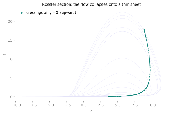
poincare_section does this for a live system. We first settle onto the attractor (so the transient does not pollute the section), then section the Rössler flow on the plane $y = 0$, keeping only upward crossings:

import numpy as np
import tsdynamics as ts

ros = ts.systems.Rossler()          # a=0.2, b=0.2, c=5.7 — the classic chaotic band

section = ts.poincare_section(
    ros,
    plane=("y", 0.0, "up"),         # section y = 0, crossed with ẏ > 0
    n=500,
    dt=0.02,
    seed=0,
)

section.summary()
# PoincareSection  (Rossler)
#   crossings = 500
#   dim = 3
#   plane = (1, 0.0)
#   direction = up (+)

section.y[:3, [0, 2]]               # (x, z) at the first three crossings
# array([[1.2932, 0.0449],
#        [2.3779, 0.0578],
#        [4.3606, 0.1081]])

The plane=("y", 0.0, "up") spelling names the axis by its variables entry and gives the direction as a word; ("y", 0.0) alone, an index (1, 0.0), or a general (normal, offset) all work too (see the Poincaré reference). The return value is a PoincareSection — a Trajectory subclass carrying the full-dimensional crossing states plus a .summary() / .to_dict() / .plot surface.

Under the hood this marches the whole attractor and refines every crossing with cubic Hermite interpolation in a single Rust engine call — roughly two orders of magnitude faster than a per-dt Python loop.

FIG 1 · the Rössler flow (faint indigo, $x$–$z$ projection) crossed by the plane $y = 0$. The teal crossings collapse from the full band onto a thin, near-one-dimensional sheet — the geometric statement that the attractor is almost two-dimensional, and its section almost a curve. That near-1-D-ness is what makes the return map in §3 single-valued.

2. The section as a discrete map¶

The same section is also a derived system you can hand to any map analysis. PoincareMap wraps the flow and presents crossing $n \mapsto$ crossing $n+1$ as a DiscreteMap-shaped object:

pmap = ts.PoincareMap(ros, plane=("y", 0.0, "up"))

sec = pmap.trajectory(500, transient=50, ic=[1.0, 1.0, 1.0])
len(sec.y)              # 500 crossings (after discarding the first 50)

Here transient counts crossings to discard, not time — the glossary distinction that keeps section transients separate from integration transients. Because a PoincareMap is a map, you can drive the whole discrete toolkit through it. An orbit_diagram over a control parameter of the wrapped flow, for instance, is a genuine bifurcation diagram of the flow — the period-doubling cascade you would otherwise have to read off by eye:

od = ts.orbit_diagram(pmap, "c", np.linspace(3.0, 6.0, 200),
                      component=0, transient=100, n=80, ic=[1.0, 1.0, 1.0])
od.bifurcation_points()[:3]     # where the cascade branches

3. The first-return map¶

Sectioning gives full crossing states; the return map goes one step further and plots a single observable at successive crossings against itself — $v_{n+1}$ vs $v_n$ — the literal 1-D map. return_map with method="poincare" does this on the same section:

rm = ts.return_map(ros, "x", method="poincare",
                   plane=("y", 0.0), direction=+1,
                   n=500, dt=0.02, seed=0)

len(rm)                 # 499  — one pair per consecutive crossing
rm.current[:3]          # array([1.2932, 2.3779, 4.3606])   (x_n)
rm.successor[:3]        # array([2.3779, 4.3606, 7.8082])   (x_{n+1})

rm.current / rm.successor are the scatter arrays $(x_n, x_{n+1})$; iterate rm for the pairs, or call rm.flat(). The result renders itself — rm.to_plot_spec() builds a return_map scatter with the fixed-point diagonal $v_{n+1} = v_n$ drawn in, and rm.cobweb() gives the cobweb-plot variant.

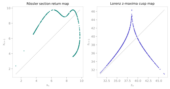
Plotted (Fig 2, left) the Rössler return map is a single-valued curve with one smooth hump — the flow's chaos is organised by an effectively one-dimensional, noninvertible map, exactly as the thin section in Fig 1 promised.

4. The Lorenz z-maxima cusp¶

Lorenz's original 1963 construction did not even need a section: he recorded the successive local maxima of $z$ and plotted each against the next. Do the same with method="max" (the default), on the Lorenz attractor, again settling first:

lor = ts.systems.Lorenz()
ic = lor.integrate(final_time=40.0, dt=0.01, ic=[1.0, 1.0, 1.0]).y[-1]
# ic ≈ [4.369, 1.717, 26.335]  — a point on the attractor

zc = ts.return_map(lor, "z", method="max", n=2000,
                   final_time=400.0, dt=0.01, ic=ic)

len(zc)                 # 532  — that many z-maxima in 400 time units
zc.values.min(), zc.values.max()   # (30.976, 46.366)  — the range of maxima
zc.current[:3]          # array([36.488, 38.309, 43.115])   (z_n^max)
zc.successor[:3]        # array([38.309, 43.115, 34.766])   (z_{n+1}^max)

Plotted (Fig 2, right), the 532 pairs fall on a sharp tent — the famous cusp map. This is Lorenz's punchline: the strange attractor, for all its apparent complexity, hides a one-dimensional map with a single unstable fixed point (where the curve crosses the diagonal) whose slope exceeds one in magnitude everywhere — the analytic fingerprint of chaos. return_map sharpens each maximum by parabolic interpolation, so a coarse dt still lands the peaks accurately.

Two return maps: Rössler section return set (left) and the Lorenz z-maxima cusp (right) — FIG 2 · first-return maps of two flows, each with the diagonal $v_{n+1}=v_n$ dashed. **Left:** the Rössler section's $x$-return map (teal) — a single-valued unimodal curve. **Right:** the Lorenz $z$-maxima cusp (indigo) — the sharp tent Lorenz drew in 1963. Where each curve crosses the diagonal is an unstable fixed point of the reduced 1-D dynamics; the steep slope there is the mechanism of the chaos.

Reading the result¶

A tight, single-valued curve (both panels of Fig 2) means the asymptotic motion is effectively governed by a 1-D map — you can study the flow's chaos with the entire theory of one-dimensional maps (fixed points, their slopes, the orbit diagram, symbolic dynamics).
A filled, multi-valued cloud means it is not 1-D — the section is genuinely two- or higher-dimensional, and the return map is only a projection. That is itself diagnostic: it says the attractor's dimension exceeds two by more than a little.
Extrema vs Poincaré. method="max"/"min" need no plane — they read peaks of one coordinate (Lorenz's construction). method="poincare" reads the observable at section crossings and needs a plane. Use extrema when a coordinate has clean, well-separated maxima; use a section when it does not, or when you want the crossings for other analyses too.

Pitfalls¶

Situation	What to do
First crossings look transient	Settle first (integrate, take `y[-1]` as `ic`) or pass `skip_crossings=` / `transient=` (crossings, not time).
Return map is a fuzzy band, not a curve	The attractor is not near-1-D on this observable — try a different component, or accept it as evidence of higher dimension.
`dt` too coarse, peaks missed	In `method="poincare"` `dt` only has to not skip a crossing; in extremum mode the peak is parabolically sharpened, so a coarse grid is usually fine — but a `dt` larger than the oscillation will still lose maxima.
Section on a stiff / DDE flow	The engine fast path needs a numeric RHS and an explicit method; stiff defaults, DDEs and `backend="reference"` fall back to the (correct, slower) Python loop automatically.