Visualization

Visualization

Every plot TSDynamics produces is described once, as a backend-agnostic PlotSpec — a semantic, JSON-serializable intermediate representation of a figure — and rendered on demand by any of four pluggable backends. Describe the Lorenz attractor once and the same object becomes a vector PDF for a paper, an interactive rotatable page for a talk, a WebGL viewer for a website, or a data payload for a custom pipeline. Nothing about the description changes; only the renderer does.

This is the module people reach for when a result has to leave the notebook — into a manuscript, a slide, a poster, a supplementary web page. It is built for that: the same spec renders identically across backends, the styling vocabulary is validated up front (a typo warns, it does not silently vanish), and every figure the system catalogue ships was produced through exactly this path.

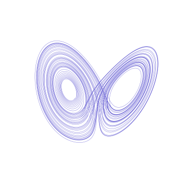
One PlotSpec, one line: ts.systems.Lorenz(ic=[1,1,1]).plot(kind="phase_portrait_3d"). The axes are hidden with .style(axes=False) and the camera framed with .camera(elev=22, azim=-60) for the attractor "floating in space".

…and the same spec becomes a movie by attaching one directive — a reveal comet, a spinning attractor, or a field replaying over time:

A reveal comet — animate=True + a fading trail.

A field movie — kind="field", animate=True.

Both loops are built through the same to_plot_spec front door — see Animation. The Lorenz 3-D attractor is also a live, orbitable WebGL viewer.

Why an intermediate representation?

Most plotting APIs bind you to one library the moment you call them: a matplotlib figure cannot become an interactive page, a plotly figure cannot be diffed or cached as data. TSDynamics splits the two concerns that libraries conflate.

• What to draw — a semantic description: this is a 3-D phase portrait, with one line layer, coloured by elapsed time, on equal axes. That is the PlotSpec. It holds NumPy arrays and typed presentation metadata, and imports no plotting library.
• How to draw it — a renderer consumes the spec. matplotlib for paper-ready raster/vector output, plotly for interactive HTML, three.js for WebGL viewers, JSON for a raw data export.

Three properties fall straight out of the split, and all three matter for research work:

1. Backend independence. A tweak like .rescale(x="log") or .recolor("#11857A") touches the spec, not a renderer, so it renders identically on every backend. Compose your figure once; export it four ways.
2. Serialisation. spec.to_dict() round-trips the whole figure — arrays, axes, colorbar, annotations — to plain JSON and back via PlotSpec.from_dict(...). A computed spec can be cached, version-controlled, shipped to a web frontend, or replotted months later without rerunning the analysis.
3. Zero import cost. A plain import tsdynamics pulls in no plotting library. ts.viz is bound lazily and each renderer's import is deferred to its first render, so the core library stays light on a headless cluster.

import tsdynamics as ts

# Build the spec once (no plotting library imported yet)…
spec = ts.systems.Lorenz(ic=[1.0, 1.0, 1.0]).to_plot_spec()

spec.save("lorenz.pdf")     # → matplotlib: a vector figure for a manuscript
spec.save("lorenz.html")    # → plotly: a self-contained interactive page
spec.save("lorenz.json")    # → the raw data payload

blob = spec.to_dict()                 # plain JSON — cache it, ship it, diff it
same = ts.viz.PlotSpec.from_dict(blob)  # rebuilt, no recomputation

The architecture

        your system / trajectory / analysis result
                          │
                 to_plot_spec(...)        ← the front door (one panel)
                          │
                          ▼
    ┌───────────────────────────────────────────────┐
    │                  PlotSpec (IR)                  │
    │  kind · layers · axes · colorbar · legend ·     │
    │  theme · annotations · animation · meta         │
    └───────────────────────────────────────────────┘
        │            │            │            │
   matplotlib      plotly      three.js       json
   (raster/       (interactive  (WebGL       (data
    vector)         HTML)       viewer)      export)

• PlotSpec — the top-level object. It carries a semantic PlotKind (what the plot means), a list of drawable Layers (each a mark plus its channel arrays), typed x/y/z Axis objects, an optional Colorbar and Legend, a Theme, Annotations (reference lines the result carries — a logistic period-doubling onset, a fit region), and an optional Animation.
• PlotKind — a closed, reviewed vocabulary of plot kinds (TIME_SERIES, PHASE_PORTRAIT_2D/_3D, SPACETIME, SPATIAL_FIELD, BIFURCATION, RECURRENCE_PLOT, …) and layer marks (LINE, SCATTER, IMAGE, SURFACE3D, …). Adding a renderer never needs a new kind; adding a kind is a deliberate contract change.
• Renderers — matplotlib is the universal reference backend (it draws every kind and is the default), plotly adds interactive 2-D/3-D and HTML animation, threejs exports a WebGL attractor viewer, and json serialises. Dispatch selects a backend by name or by capability, and falls back to matplotlib with a VisualizationDegraded warning when a partial backend declines a kind — so a figure never silently fails to render.

A map of this section

• Plotting — the front door

  ---

  traj.to_plot_spec / .plot: the auto-dispatch on component count, the PlotKind vocabulary (time series · 2-D & 3-D phase portraits · spacetime · delay embeddings · spatial fields), components= selection, and per-kind options — every kind with a runnable, IC-pinned example.

• Figure conventions

  ---

  The rules the catalogue figures follow — viridis for sequential fields, twilight for cyclic ones, the teal/indigo brand accents, one figure per concept, colorbars and legends — so your figures come out paper-ready.

• Styling & themes

  ---

  The canonical per-layer style vocabulary (STYLE_KEYS + normalize_style), the fluent chainable tweaks (.style / .recolor / .theme / .grid / .background / …), the four built-in themes, and the per-backend honoring contract.

• Animation

  ---

  Animation as an orthogonal modifier — .animate / .trail / .head / .camera / .clock, the reveal comet vs the frames spatial-field movie, and export to .mp4 / .gif (matplotlib) or a live .html comet (plotly).

• Composition

  ---

  ts.viz.plot(...): overlay compatible panels on one set of axes, or tile them with layout="stack"/"row"/"grid" — a spec-in / spec-out figure-level front door that composes recursively.

• Backends & export

  ---

  The four renderers (matplotlib · plotly · json · three.js), how dispatch and fallback work, spec.save(path) by extension, and the self-contained interactive WebGL three.js export that ships on the 3-D catalogue pages.

Three ways in

There is a single conceptual pipeline, but three surfaces onto it depending on how much you want to say.

One-linerBuild, tweak, renderCompose panels

.plot() on any system, Trajectory, or analysis result builds the spec and renders it in one call:

import tsdynamics as ts

ts.systems.Rossler(ic=[1.0, 1.0, 1.0]).plot()   # auto-dispatched view

A system's .plot() integrates with sensible defaults first; a Trajectory's plots the data you already have.

Keep the spec, chain fluent tweaks, then render or save. Every tweak mutates the spec and returns it, so they compose:

import tsdynamics as ts

traj = ts.systems.Rossler(ic=[1.0, 1.0, 1.0]).integrate(final_time=200, dt=0.05)
(
    traj.to_plot_spec(components=["x", "y"], color_by="time")
        .relabel(title="Rössler")
        .grid()
        .save("rossler.pdf")
)

ts.viz.plot(*things, layout=...) arranges multiple things into one figure — overlaid on shared axes, or tiled into panels — and returns a spec that itself renders:

import tsdynamics as ts

a = ts.systems.Lorenz(ic=[1.0, 1.0, 1.0]).integrate(final_time=100, dt=0.01)
b = ts.systems.Rossler(ic=[1.0, 1.0, 1.0]).integrate(final_time=200, dt=0.05)
ts.viz.plot(a, b, layout="grid").save("two-attractors.pdf")

Installing a backend

The IR ships with the core library; a backend is an optional extra you install when you want to render:

Extra	Backend	Draws
tsdynamics[viz]	matplotlib	everything — raster (.png/.jpg) and vector (.pdf/.svg), plus .mp4/.gif animation
tsdynamics[interactive]	plotly	interactive 2-D/3-D HTML, real-time animated .html
(bundled)	json, three.js	data export — no plotting dependency

With no backend installed, spec.to_dict() still works — you can render the payload yourself. Once matplotlib is present it becomes the default for everything, and .save(path) picks the right backend from the file extension.

See also

• Plotting — the front door — start here to make your first figure.
• Tutorials — end-to-end journeys that dogfood this module.
• PlotSpec reference — the full IR surface.