Tutorial · Noise-driven dynamics

Noise-driven dynamics¶

Add noise to a dynamical system and the questions change. A single trajectory is no longer the answer — it is one draw from a distribution, and the useful objects become statistical: the ensemble mean, the stationary variance, the rate at which noise kicks the state over a barrier. TSDynamics models these as diagonal-Itô SDEs,

\[dX_k = f_k(X, t)\,dt + g_k(X, t)\,dW_k,\]

a deterministic drift $f$ (the skeleton, exactly like an ODE's _equations) plus an independent Wiener increment $dW_k$ scaled by a diffusion coefficient $g_k$. This tutorial walks the three things you actually do with one: integrate a path, gather ensemble statistics, and study noise-induced transitions — checking each against the analytic law and the deterministic limit.

Every number below is reproducible: paths and ensembles are seeded, and each printed value is what the shown code returns.

1. A single path¶

The catalogue ships three canonical processes in the sde family. Start with the Ornstein–Uhlenbeck process — additive-noise mean reversion, the continuous AR(1),

\[dX = \theta\,(\mu - X)\,dt + \sigma\,dW,\]

a linear restoring drift pulling the state to the mean $\mu$ at rate $\theta$ against constant Gaussian noise. Integrate one realisation. The seed fixes the noise so the path is reproducible, and dt sets both the output grid and the noise scale $\sqrt{dt}$:

import numpy as np
import tsdynamics as ts

ou = ts.systems.OrnsteinUhlenbeck(params={"theta": 1.0, "mu": 0.0, "sigma": 0.3})

path = ou.integrate(final_time=30.0, dt=0.01, ic=[2.0], seed=0)

path.y.shape            # (3001, 1)
path.y[0, 0]            # 2.0   — the initial condition
round(path.y[-1, 0], 4) # 0.2887 — where this particular realisation ended
path.meta["method"]     # 'euler_maruyama'  (the default scheme)
path.meta["seed"]       # 0  — recorded for reproducibility

The path starts at $x_0 = 2$, is pulled toward $\mu = 0$, and then rattles around it. The OU process has a known stationary distribution — normal with mean $\mu$ and variance $\sigma^2 / 2\theta$ — so once the transient has died the path statistics should match it. Read them off the tail of this single long run:

0.3**2 / (2 * 1.0)              # 0.045   — analytic stationary variance
tail = path.y[path.t > 10.0, 0]
round(tail.mean(), 4)          # -0.0297  ≈ μ = 0
round(tail.var(), 4)           # 0.0365   ≈ 0.045 (one path — noisy estimate)

One path gives a noisy variance estimate ($0.037$ vs the true $0.045$). To pin the statistics down we need many paths.

Euler–Maruyama vs Milstein

method="euler_maruyama" (order 0.5, the default) is the workhorse; method="milstein" (order 1.0) adds a correction proportional to $g\,\partial g/\partial x$. For additive noise ($g$ constant, as in OU and the double well) that correction is identically zero, so the two schemes produce bit-identical paths — a useful sanity check. Milstein only differs for multiplicative noise (§4's geometric Brownian motion).

2. Ensemble statistics¶

The right object for a stochastic system is the ensemble. ou.ensemble(...) integrates a batch of initial conditions and returns each one's final state, fanning the batch out across the compiled engine's thread pool:

ics = np.full((2000, 1), 2.0)          # 2000 copies of the same start
finals = ou.ensemble(ics, final_time=30.0, dt=0.01, seed=0)

finals.shape                            # (2000, 1)
round(finals.mean(), 4)                 # -0.0007  ≈ μ = 0
round(finals.var(), 4)                  # 0.0451   ≈ 0.045  — the analytic variance
int(np.isnan(finals).any(axis=1).sum()) # 0  — no diverged trajectories

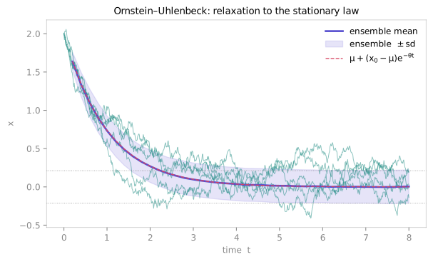
With 2000 paths the ensemble variance at $T = 30$ nails the stationary value $0.045$. The transient matches theory too: the ensemble mean decays as $\mu + (x_0 - \mu)\,e^{-\theta t}$. Sweep the horizon and compare:

for T in (0.5, 1.0, 2.0):
    f = ou.ensemble(ics, final_time=T, dt=0.01, seed=0)
    print(f"T={T}: mean={f.mean():.4f}  analytic={2.0*np.exp(-T):.4f}")
# T=0.5: mean=1.2071  analytic=1.2131
# T=1.0: mean=0.7299  analytic=0.7358
# T=2.0: mean=0.2689  analytic=0.2707

Three decimals of agreement, from the raw ensemble against the closed-form transient.

OU sample paths with the ensemble mean tracking the analytic exponential decay and a ±sd band — FIG 1 · Ornstein–Uhlenbeck relaxation. Five seeded sample paths (faint teal) start at $x_0 = 2$ and are pulled toward $\mu = 0$. The ensemble mean (indigo, over 3000 paths) tracks the analytic transient $\mu + (x_0-\mu)e^{-\theta t}$ (dashed rose) exactly, while the $\pm\,$sd band (indigo shading) widens to the stationary spread $\sigma/\sqrt{2\theta}$ (dotted). The single path is one draw; the ensemble is the law.

Ensemble seeding is by index — by design

ensemble(ics, seed=s) seeds trajectory $i$ from seed_for(s, i), a mix depending only on the index, so the batch is reproducible and matches the engine's parallel-equals-serial contract. This means ensemble([ic], seed=s) generally draws a different sample path from integrate(seed=s) for the same s — they are different streams. (The one coincidence: seed_for(0, 0) happens to be 0, so at seed=0 index 0 alone they align.) Do not expect ensemble and integrate to reproduce each other path-for-path; do expect each, on its own, to reproduce exactly under a fixed seed.

3. Noise-induced switching (Kramers escape)¶

Now the headline stochastic phenomenon. The double-well process is overdamped gradient flow in the bistable potential $U(x) = -\tfrac{a}{2}x^2 + \tfrac{b}{4}x^4$,

\[dX = (a\,X - b\,X^3)\,dt + \sigma\,dW,\]

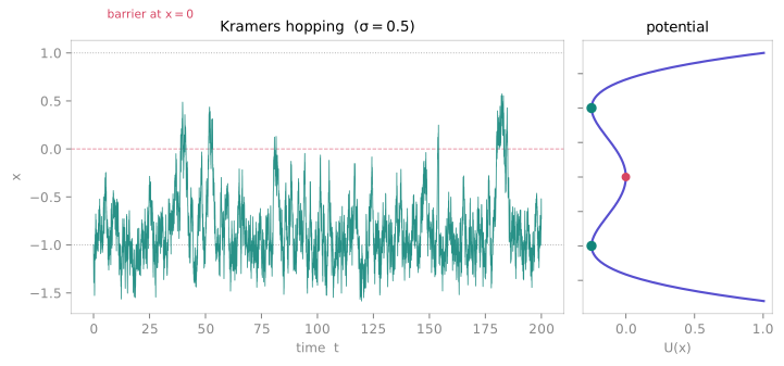
with stable wells at $x = \pm\sqrt{a/b} = \pm 1$ separated by a barrier at the origin. Without noise the state relaxes into whichever well it starts in and stays there forever. With noise it occasionally hops the barrier — the long-time dynamics is a random telegraph between the two wells. Integrate a long path starting in the left well:

dw = ts.systems.DoubleWell(params={"a": 1.0, "b": 1.0, "sigma": 0.5})
path = dw.integrate(final_time=200.0, dt=0.01, ic=[-1.0], seed=1)
x = path.y[:, 0]

# barrier hops = sign changes of x (the state crossing x = 0)
int(np.sum(np.diff(np.sign(x)) != 0))   # 70   — this realisation hops 70 times
round((x < 0).mean(), 3)                # 0.962 — but spends 96% of its time left

The path hops 70 times yet lives mostly in the left well: it starts there, and at $\sigma = 0.5$ each escape is rare enough that it mostly falls back. The escape rate is governed by Kramers' law — the mean residence time is exponential in the barrier-height-to-noise ratio, $\sim \exp(2\,\Delta U / \sigma^2)$ — so a modest increase in $\sigma$ multiplies the hopping. Turn the noise up and count again:

x8 = ts.systems.DoubleWell(params={"a": 1.0, "b": 1.0, "sigma": 0.8}) \
        .integrate(final_time=200.0, dt=0.01, ic=[-1.0], seed=1).y[:, 0]
int(np.sum(np.diff(np.sign(x8)) != 0))  # 324  — 4.6× the hops of σ = 0.5

Double-well telegraph path hopping between wells, beside the double-well potential — FIG 2 · noise-induced switching in the double well ($\sigma = 0.5$). **Left:** a single 200-time-unit path (teal) rattling in the wells at $x = \pm 1$ and occasionally hopping the barrier at $x = 0$ (dashed rose). **Right:** the potential $U(x)$, with the two stable minima (teal) and the unstable barrier (rose) the noise must climb. Raising $\sigma$ lowers the effective barrier-to-noise ratio and the hopping proliferates (Kramers).

The ensemble view makes the metastability quantitative: start 4000 paths in the left well and, after long enough, they redistribute toward the symmetric $\tfrac12 / \tfrac12$ occupation of the two wells:

ics = np.full((4000, 1), -1.0)
finals = dw.ensemble(ics, final_time=50.0, dt=0.01, seed=0)
finals = finals[~np.isnan(finals).any(axis=1)]
round((finals[:, 0] > 0).mean(), 3)     # 0.472 — nearly half have escaped to the right well

4. Multiplicative noise: geometric Brownian motion¶

Not all noise is additive. Geometric Brownian motion — the Black–Scholes asset-price model — scales both drift and diffusion with the state,

\[dX = \mu\,X\,dt + \sigma\,X\,dW,\]

so its log is a Brownian motion with drift, the path stays strictly positive, and the ensemble is log-normal. Its mean grows as $X_0\,e^{\mu t}$ while its median grows more slowly, as $X_0\,e^{(\mu - \sigma^2/2)t}$ — the gap is the signature of multiplicative noise. Check both against the ensemble:

gbm = ts.systems.GeometricBrownianMotion(params={"mu": 0.1, "sigma": 0.3})
finals = gbm.ensemble(np.full((5000, 1), 1.0), final_time=5.0, dt=0.005, seed=0)
finals = finals[~np.isnan(finals).any(axis=1)]

round(finals.mean(), 4)                 # 1.6585  vs  exp(μT)          = 1.6487
round(float(np.median(finals)), 4)      # 1.3356  vs  exp((μ-σ²/2)T)   = 1.3165
bool((finals > 0).all())                # True   — every path stayed positive

Because $g = \sigma X$ is state-dependent, this is where Milstein actually differs from Euler–Maruyama — for a serious moment estimate at coarse dt, prefer method="milstein".

5. The deterministic skeleton¶

Every SDE contains an ODE: set $\sigma = 0$ (or read the drift alone) and you have the deterministic skeleton that the noise perturbs. It is always worth looking at — it tells you where the attractors of the noisy system are hiding. For the double well the skeleton is a bistable gradient flow: without noise the state simply rolls into the nearest well and stops.

det = ts.systems.DoubleWell(params={"a": 1.0, "b": 1.0, "sigma": 0.0})

round(det.integrate(final_time=50.0, dt=0.01, ic=[-1.5], seed=0).y[-1, 0], 4)  # -1.0
round(det.integrate(final_time=50.0, dt=0.01, ic=[ 0.2], seed=0).y[-1, 0], 4)  #  1.0

From $x_0 = -1.5$ it settles into the left well ($-1$); from $x_0 = 0.2$, just right of the barrier, into the right well ($+1$). Those two fixed points are exactly the states the noise telegraphs between in §3 — the skeleton's basins (which you can map with basins_of_attraction on the $\sigma = 0$ system) are the wells; the noise supplies the barrier-hopping the skeleton can never do on its own.

Skeleton first, then noise

A good workflow for any SDE: study the deterministic skeleton with the full ODE toolkit — fixed points, Lyapunov exponents, basins — to map the landscape, then add noise and ask how it moves the state around that landscape. The stochastic phenomena (escape, resonance, noise-induced transitions) are all statements about noise versus that fixed geometry.

What you built¶

You integrated a single stochastic path, gathered an ensemble whose statistics matched the analytic OU laws to three decimals, watched noise drive Kramers escape across a double-well barrier (and proliferate as $\sigma$ grew), confirmed the log-normal mean/median gap of multiplicative noise, and grounded all of it in the deterministic skeleton underneath. Each result carries its scheme, seed and dt in .meta, so any path or ensemble replays exactly.