Theory

Solvers & methods

Most of the time you never touch this layer. You call run() and the default solver does the right thing:

import tsdynamics as ts

traj = ts.systems.Lorenz().run(final_time=100.0, dt=0.01)

When you do want to choose — a stiff chemical model, a high-accuracy reference run, a fixed-step orbit — you pass a method= string:

traj = ts.systems.Lorenz().run(final_time=100.0, dt=0.01, solver="dop853")

This page is the catalogue of those names and a guide to picking one. Every method below is a thin Python spec (SolverSpec) mirroring a kernel in the Rust engine; the string you pass is normalised, alias-mapped and validated against a registry before the engine runs it. For the programmatic registry API (resolving names, capability flags, registering your own) see Reference → Solvers.

dt is the output grid, not the step size

For every adaptive method, dt only sets how densely the returned Trajectory is sampled — the internal stepper chooses its own steps from rtol/atol. A coarse dt does not cost accuracy. The two exceptions are rk4 (a genuinely fixed-step method, where dt is the step) and the stochastic schemes (where dt is the noise increment \(\sqrt{\mathrm{d}t}\)).

Since rtol is therefore the only accuracy knob, v6 tightened its default to 1e-9 (atol=1e-12) — see the tolerance table.

The catalogue

method=	Family	Kind	Order	Adaptive	Needs Jacobian	Use when
euler	ode, dde	explicit RK (fixed)	1	—	—	the simplest baseline; teaching
midpoint	ode, dde	explicit RK (fixed)	2	—	—	a cheap fixed-step march
heun	ode, dde	explicit RK (fixed)	2	—	—	explicit trapezoid / improved Euler
ralston	ode, dde	explicit RK (fixed)	2	—	—	min-error-bound order-2 fixed step
ssprk3	ode, dde	explicit SSP RK (fixed)	3	—	—	TVD/SSP march for hyperbolic MOL discretisations
rk4	ode, dde	explicit RK (fixed)	4	—	—	a fixed-step march; teaching; debugging step effects
rk4_38	ode, dde	explicit RK (fixed)	4	—	—	the 3/8-rule RK4 (smaller error constant)
ab3 / ab4	ode, dde	explicit Adams–Bashforth (multistep)	3 / 4	—	—	non-stiff with an expensive RHS (1 eval/step); MOL/spectral systems
abm4	ode, dde	Adams–Bashforth–Moulton (PECE)	4	—	—	non-stiff, more accuracy/stability than ab4 (2 evals/step)
heun_euler	ode, dde	explicit RK (embedded)	2(1)	✓	—	the cheapest adaptive kernel; coarse tolerances
bs3	ode, dde	explicit RK (embedded)	3(2)	✓	—	crude–moderate tolerances (the ode23 pair)
rk45	ode, dde	explicit RK (embedded)	5(4)	✓	—	the default — non-stiff smooth problems
rkf45	ode, dde	explicit RK (embedded)	5(4)	✓	—	the classic Runge–Kutta–Fehlberg pair
cashkarp	ode, dde	explicit RK (embedded)	5(4)	✓	—	non-stiff; rapidly-varying RHS
tsit5	ode, dde	explicit RK (embedded)	5(4)	✓	—	non-stiff, often fewer evaluations than rk45
dop853	ode, dde	explicit RK (embedded)	8(5,3)	✓	—	high accuracy / tight tolerances; reference runs
bdf	ode	implicit (multistep)	1–5 var.	✓	✓	the stiff default — smooth stiff RHS
backward_euler	ode	implicit (backward Euler)	1	✓	✓	the canonical L-stable stiff baseline
implicit_midpoint	ode	implicit (1-stage Gauss)	2	✓	✓	A-stable order-2 (base step symplectic; see note below)
trapezoid	ode	implicit (Crank–Nicolson)	2	✓	✓	mildly-stiff oscillatory problems (A-stable)
sdirk2	ode	implicit (SDIRK)	2	✓	✓	stiff, L-stable 2-stage SDIRK
rosenbrock	ode	implicit (Rosenbrock-W)	fixed	✓	✓	stiff, one linear solve per step
trbdf2	ode	implicit (ESDIRK)	2	✓	✓	stiff, L-stable composite step
euler_maruyama	sde	explicit	0.5 (strong)	—	—	the SDE default — diagonal-Itô noise
milstein	sde	explicit	1.0 (strong)	—	✓ (∂g/∂u)	SDE, higher strong order

All names are case- and punctuation-insensitive and carry common aliases (e.g. dopri5/RK45 → rk45, ode23 → bs3, cash_karp → cashkarp, crank_nicolson → trapezoid, implicit_euler → backward_euler, adams_bashforth/ab → ab4). The list is open: new kernels register themselves (see Programmatic registry).

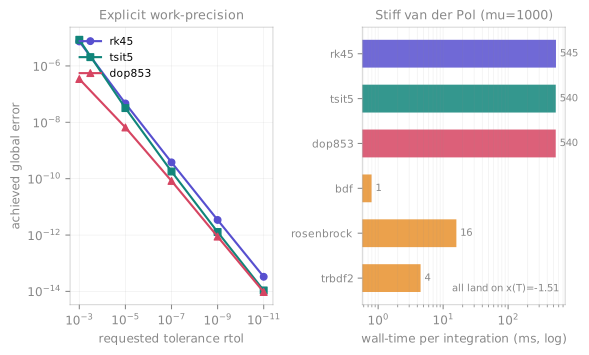
Left: on a scalar problem with a known solution the explicit kernels track the requested tolerance, with the order-8 dop853 reaching the lowest error at every setting. Right: on stiff van der Pol (μ=1000) all six kernels land on the same final state, but the explicit methods are stability-bound and pay hundreds of times the wall-time of the implicit ones — the practical case for bdf.

Explicit Runge–Kutta

These are the workhorses for smooth, non-stiff problems, and the same kernels drive the DDE families through the method of steps. The family spans fixed-step methods from order 1 (euler) through the order-4 rk4/rk4_38, the SSP order-3 ssprk3, the embedded adaptive pairs (heun_euler, bs3, rk45, rkf45, cashkarp, tsit5, dop853), and the explicit Adams–Bashforth multistep methods (ab3, ab4, abm4). Pick a fixed-step method when you want a deterministic step count, a low-order one for teaching, and an adaptive pair for production non-stiff integration.

rk4 is the classic four-stage, fourth-order Runge–Kutta with a fixed step (Kutta 1901): no embedded error estimate, no adaption. Pass it when you want a deterministic step count or to study how step size affects a result — for production integration prefer an adaptive method. The low-order fixed kernels euler (Euler 1768), midpoint/heun/ralston (order 2) and the SSP ssprk3 (Shu & Osher 1988, the standard time integrator for hyperbolic PDE discretisations) round out the fixed-step set.

The Adams–Bashforth multistep kernels (ab3/ab4) and the Adams–Bashforth–Moulton predictor–corrector (abm4) reuse right-hand-side values from previous steps, so they advance with only one (ab*) or two (abm4) new RHS evaluations per step regardless of order — efficient when f is expensive, as in the large ODE systems from method-of-lines/spectral discretisations of PDEs (Adams 1883; Hairer, Nørsett & Wanner 1993, §III.1). They are fixed-step and self-start with rk4. (For genuinely stiff semilinear PDEs such as Kuramoto–Sivashinsky, an explicit Adams method is stability-bound; the efficient route is an implicit/IMEX or exponential-integrator split of the linear and nonlinear operators — a future seam, since the present engine takes a single combined f(u, t).)

# Fixed-step march: dt IS the integrator step here.
traj = ts.systems.Lorenz().run(final_time=20.0, dt=0.005, solver="rk4")

rk45 is the embedded Dormand–Prince 5(4) pair (Dormand & Prince 1980) and the default for ODEs and DDEs. The fifth-order solution advances the state and the embedded fourth-order solution estimates the local error, which drives the adaptive step controller. Spellings dopri5 and RK45 resolve to it.

# All four lines integrate with the same kernel.
ts.systems.Rossler().run(final_time=200.0, dt=0.05)                 # default
ts.systems.Rossler().run(final_time=200.0, dt=0.05, solver="rk45")
ts.systems.Rossler().run(final_time=200.0, dt=0.05, solver="dopri5")
ts.systems.Rossler().run(final_time=200.0, dt=0.05, solver="RK45")

tsit5 is Tsitouras' 5(4) pair (Tsitouras 2011), an explicit RK with coefficients optimised to minimise the leading truncation-error term. It is another excellent general-purpose non-stiff choice and frequently spends fewer right-hand-side evaluations than rk45 at the same tolerance.

dop853 is the eighth-order Dormand–Prince method with embedded fifth- and third-order estimators for stepsize control (Hairer, Nørsett & Wanner 1993). Reach for it when you need tight tolerances or a high-accuracy reference trajectory — at small rtol it reaches a far lower error than the 5(4) pairs for comparable work (the left panel above).

# High-accuracy reference run.
traj = ts.systems.Lorenz().run(
    final_time=100.0, dt=0.01, solver="dop853", rtol=1e-12, atol=1e-12
)

Implicit / stiff

A problem is stiff when its Jacobian has eigenvalues spanning many orders of magnitude: a fast-decaying mode forces an explicit method to take tiny steps for stability long after the solution itself has gone smooth. The fix is an implicit method, whose stability region covers the entire left half-plane (it is A- or L-stable), so the step size is bounded by accuracy alone. The right panel of the figure makes the cost concrete: on stiff van der Pol every kernel reaches the same final state, but the explicit methods run hundreds of times slower.

Every implicit kernel is adaptive and requires the analytic Jacobian \(\partial f/\partial u\). You never build it: the engine differentiates your _equations symbolically and lowers a Jacobian-carrying tape automatically whenever the resolved kernel needs one, so solver="bdf" simply works.

bdf is the variable-order (1–5), fixed-leading-coefficient backward differentiation formula (Curtiss & Hirschfelder 1952; Shampine & Gordon 1975) — a multistep method with its own order and step controllers. It is the default stiff method for ODEs: through a smooth stiff phase it takes far larger steps than the fixed-order one-step kernels, which is why it is the right starting point for stiff problems.

rosenbrock is a linearly-implicit Rosenbrock-W method (Rosenbrock 1963): one linear solve per step, no Newton iteration, with step-doubling + Richardson extrapolation for error control. trbdf2 is the TR-BDF2 composite single-step ESDIRK (Bank et al. 1985) — a trapezoidal sub-step followed by a BDF2 sub-step, L-stable, also step-doubling controlled. Both stay selectable by name when you want a one-step kernel instead of the multistep bdf.

The one-step stiff family is rounded out by backward_euler (implicit Euler, order 1, L-stable — the canonical stiff baseline), sdirk2 (a 2-stage L-stable singly-diagonally-implicit Runge–Kutta, Alexander 1977), and two A-stable methods: trapezoid (the Crank–Nicolson rule, Crank & Nicolson 1947) and implicit_midpoint (the one-stage Gauss collocation method, A-stable order 2; its base step is symplectic, but the adaptive integrator delivered here drives it through Richardson step-doubling, which is not symplectic, so it does not carry the long-time energy-conservation guarantee of a fixed-step symplectic method; Hairer, Lubich & Wanner 2006). All four solve their implicit stage(s) by a modified-Newton iteration reusing the analytic Jacobian, and share the step-doubling error controller. The A-stable (non-L-stable) trapezoid/implicit_midpoint can ring on the very stiffest transients — prefer an L-stable kernel (bdf, backward_euler, sdirk2, rosenbrock, trbdf2) there.

A higher-order stiff Radau IIA collocation kernel and the Verner/Feagin high-order explicit pairs are natural follow-ups; they slot in behind the same Solver seam.

Mark a system stiff once and forget it — declare the default method on the class:

class MyStiffSystem(ts.ContinuousSystem):
    _default_method = "bdf"          # every run() now uses bdf
    ...

The built-in stiff catalogue systems (for example Oregonator, the Field–Noyes Belousov–Zhabotinsky model) already do this.

LSODA, Radau, vode are not method names

The legacy SciPy/v2 stiff names have no engine kernel and are rejected on resolution, with a hint pointing at the engine's stiff family:

ts.systems.Oregonator().run(solver="LSODA")
# ValueError: unknown solver method 'LSODA'; ...
#   ('LSODA' is a SciPy/v2 stiff method with no engine kernel;
#    use 'bdf' or 'trbdf2' for stiff problems.)

Use bdf (or rosenbrock / trbdf2) instead.

Stiff DDEs

The method-of-steps reuses only the explicit ODE kernels, so a DDE's method= is explicit-only (available_for("dde") → ['dop853', 'rk4', 'rk45', 'tsit5']). The implicit kernels are ODE-only for now; method="rosenbrock" on a DDE raises.

Stochastic

The stochastic family integrates diagonal-Itô SDEs \(\mathrm{d}X_k = f_k\,\mathrm{d}t + g_k\,\mathrm{d}W_k\) with a fixed step. Here dt is load-bearing in two ways at once: it is both the output sampling interval and the discretisation step — the Wiener increment over a step has scale \(\sqrt{\mathrm{d}t}\) — so a smaller dt is the only way to a more accurate sample path.

euler_maruyama is the Euler–Maruyama scheme (strong order 0.5), the SDE default. milstein is the Milstein scheme (strong order 1.0), which adds the diffusion-derivative correction \(\partial g/\partial u\) (built automatically, like the implicit Jacobian) for a higher strong order on the same step.

Pass a seed to make the noise realisation reproducible — it is recorded in the returned trajectory's meta:

class GBM(ts.StochasticSystem):
    params = {"mu": 0.1, "sigma": 0.3}
    dim = 1

    @staticmethod
    def _drift(y, t, *, mu, sigma):
        return [mu * y(0)]

    @staticmethod
    def _diffusion(y, t, *, mu, sigma):
        return [sigma * y(0)]

a = GBM().run(final_time=1.0, dt=0.01, ic=[1.0], solver="euler_maruyama", seed=0)
b = GBM().run(final_time=1.0, dt=0.01, ic=[1.0], solver="euler_maruyama", seed=0)
assert (a.y == b.y).all()          # same seed → identical path
c = GBM().run(final_time=1.0, dt=0.01, ic=[1.0], solver="milstein", seed=0)

An ensemble(...) run seeds trajectory \(i\) from a per-index derivation of the base seed, so a batch is reproducible and the parallel result equals the serial one.

Choosing a method

For the common cases the defaults are already right:

Family	Default	Default stiff
ODE	rk45	bdf
DDE	rk45	rosenbrock (policy; not yet a resolvable DDE kernel — see above)
SDE	euler_maruyama	—

Names normalise. A method= string is lower-cased, its whitespace and hyphens collapsed, then run through an alias table before the registry lookup — so "RK45", "dopri5", "dp45" all reach rk45; "dop8" → dop853; "ros" → rosenbrock; "em" → euler_maruyama. An unrecognised name raises with the list of valid methods for the family.

Auto-stiffness. When you are unsure, ask the registry. is_stiff probes the Jacobian spectrum at one point and reports whether the stiffness ratio (fastest over slowest decay rate) crosses a threshold; recommend combines that verdict with the policy table and hands back a ready-to-use resolution:

from tsdynamics import _solvers as solvers

solvers.is_stiff(ts.systems.Oregonator(), ic=[1.0, 1.0, 1.0])   # True
solvers.is_stiff(ts.systems.Lorenz(),     ic=[1.0, 1.0, 1.0])   # False

rec = solvers.recommend(ts.systems.Oregonator(), ic=[1.0, 1.0, 1.0])
rec.name          # 'bdf'
rec.build_kwargs  # {'with_jacobian': True}

Both are one-point heuristics evaluated at the IC, meant to seed a choice rather than guarantee one — pass an explicit ic= for a reproducible verdict (a system with a random initial condition will probe a different point each call). The authoritative signal is the engine's runtime stiffness detector, which watches the rejected-step ratio once integration is underway.

Programmatic registry

The solver layer is a pluggable registry: each method is a SolverSpec with a SolverCaps (explicit/implicit, adaptive, needs-Jacobian, supported families), method= strings resolve against it, and third-party solvers register through the same entry point. If you are building on the selection machinery — listing methods, inspecting capabilities, resolving names yourself, or registering a new kernel — see the Reference → Solvers API page for SolverSpec, SolverCaps, resolve, available_for, recommend, is_stiff, build_kwargs and register.