Tutorial · The road to chaos

The road to chaos¶

The previous tutorial took a chaotic attractor apart. This one asks the sequel: where does the chaos come from? Turn one knob on a simple system and the answer unfolds as the single most famous picture in nonlinear dynamics — a stable state that splits in two, splits again, and cascades into chaos. We will draw that bifurcation diagram, land its forks on the exact parameter values the theory predicts, confirm the onset of chaos with a Lyapunov exponent, and then — the payoff — reproduce the entire route for a continuous flow, using a Poincaré section to turn the flow into a map we can sweep the same way.

1. The canonical example: the logistic map¶

The logistic map \(x_{n+1} = r\,x_n(1 - x_n)\) models a population that grows in proportion to \(r\) but is capped by crowding. It is a one-line system, and its sole parameter \(r\) is the knob. It is in the catalogue:

import numpy as np
import tsdynamics as ts

log = ts.systems.Logistic()
log.params        # ParamSet({r=3.9})
log.variables     # ('x',)

An orbit diagram records, at each value of \(r\), the set of states the orbit visits once transients have died away. One dot means a stable fixed point; two, a period-2 cycle; a filled stripe, chaos. orbit_diagram sweeps the parameter for you:

od = ts.orbit_diagram(
    ts.systems.Logistic(),
    "r", np.linspace(2.5, 4.0, 600),   # sweep the growth rate
    n=120,          # states recorded per r
    transient=500,  # steps discarded first, at every r
)

r_vals, states = od.flat()   # scatter-ready 1-D arrays
# plt.plot(r_vals, states, ",k")   # the picture below

flat() returns two aligned arrays — the parameter repeated once per recorded point, and the asymptotic state — ready to scatter. A genuine DiscreteMap like this sweeps the whole parameter array in a single Rust engine call, so a 600-value sweep is near-instant.

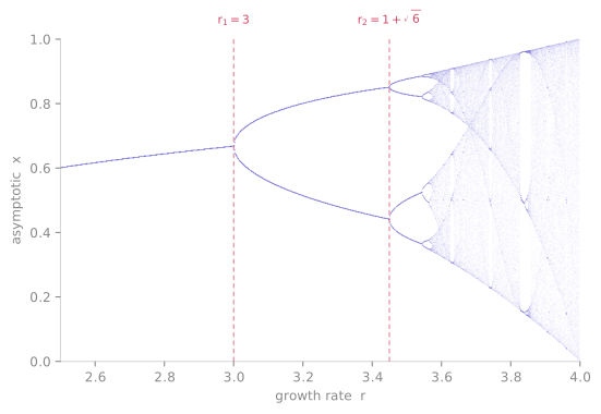
The logistic map's period-doubling bifurcation diagram over r — FIG 1 · the logistic orbit diagram. Left of r = 3 a single stable branch; at r₁ = 3 it forks to period 2, at r₂ = 1 + √6 ≈ 3.449 to period 4, then 8, 16, … accumulating at r∞ ≈ 3.5699 — the onset of chaos. Beyond it, chaotic bands threaded with periodic windows (the wide period-3 band near r ≈ 3.83).

2. How to read it — and land the onsets on the theory¶

The diagram is a route. Walk it left to right:

\(r < 3\): one branch — a single stable fixed point. The population settles to one value.
\(r_1 = 3\): the fixed point loses stability and the branch forks. The orbit now alternates between two values — period 2.
\(r_2 = 1 + \sqrt6 \approx 3.449\): each branch forks again — period 4 — then 8, 16, … in a geometric cascade that accumulates at \(r_\infty \approx 3.5699\), the onset of chaos.
beyond \(r_\infty\): mostly chaotic bands, punctured by periodic windows — most visibly a period-3 window near \(r \approx 3.83\).

Those onset values are not eyeballed off the plot — the library computes them. OrbitDiagram.periods() counts distinct branches at each \(r\) (that count is the period), and bifurcation_points() reports where the count changes:

od = ts.orbit_diagram(
    ts.systems.Logistic(), "r", np.linspace(2.9, 3.6, 400), n=64, transient=2000,
)

od.bifurcation_points()[:2]     # ≈ [3.00, 3.45]  — the first two onsets
1 + np.sqrt(6)                  #    3.4495        — matches r2 exactly

The first two forks land on the textbook values \(r_1 = 3\) and \(r_2 = 1 + \sqrt6\). The resolution of bifurcation_points() is the spacing of the swept values, so sweep finely near a transition to pin it down. And the periods themselves are exactly the doubling ladder:

od2 = ts.orbit_diagram(ts.systems.Logistic(), "r",
                       np.array([2.8, 3.2, 3.5, 3.55, 3.9]), n=64, transient=2000)
od2.periods()          # array([1, 2, 4, 8, 0])   — 0 = aperiodic (chaotic)

Period 1, 2, 4, 8, then 0 — the sentinel for a chaotic (aperiodic) orbit. The cascade, quantified.

The period-3 window

That wide band near \(r \approx 3.83\) is the period-3 window, born at the tangent bifurcation \(r = 1 + \sqrt8 \approx 3.828\) — the interval where the dynamics briefly return to order before doubling back into chaos:

ts.orbit_diagram(ts.systems.Logistic(), "r",
                 np.array([3.82, 3.83, 3.84]), n=90, transient=3000).periods()
# array([0, 3, 3])   — aperiodic, then the period-3 window opens

"Period 3 implies chaos" (Li & Yorke, 1975): the existence of a period-3 orbit forces orbits of every period and an uncountable set of aperiodic ones.

3. Confirm the onset with a Lyapunov exponent¶

The orbit diagram shows chaos as a filled band; the Lyapunov exponent measures it. For a map, \(\lambda\) is negative on a stable cycle (nearby orbits converge onto it) and positive in chaos (they diverge). Sweep it and watch the sign flip exactly where the diagram turns chaotic:

for r in [2.9, 3.2, 3.5, 3.57, 3.83, 3.9, 4.0]:
    lam = float(np.asarray(
        ts.systems.Logistic(params={"r": r}, ic=[0.1]).lyapunov_spectrum(steps=30000)
    )[0])
    print(f"r={r}: lambda = {lam:+.4f}")

# r=2.9 : lambda = -0.1054     stable fixed point
# r=3.2 : lambda = -0.9158     period 2
# r=3.5 : lambda = -0.8717     period 4
# r=3.57: lambda = +0.0112     onset of chaos — lambda crosses zero
# r=3.83: lambda = -0.3680     period-3 window — order returns, lambda dips back negative
# r=3.9 : lambda = +0.4960     chaos
# r=4.0 : lambda = +0.6931     = ln 2, the exact analytic value

\(\lambda\) is negative throughout the periodic regime, crosses zero right at the accumulation point \(r_\infty \approx 3.57\), goes positive in the chaotic bands — and dips back below zero inside the period-3 window, exactly matching the return to order the diagram shows. At \(r = 4\) it hits \(\ln 2 \approx 0.693\), the one value known in closed form (the map is conjugate to a tent map there). The picture and the number tell the same story.

4. The same route, for a flow¶

Nothing about the cascade is special to maps. A continuous system period-doubles its way to chaos too — you just cannot sweep a flow directly, because a flow has no discrete "next state" to record. The derived wrappers fix that: a PoincareMap samples the flow only where it pierces a chosen plane, presenting it as a genuine discrete map. Sweeping a parameter of that is the bifurcation diagram of the flow.

We use the Rössler system — three equations whose single parameter \(c\) drives exactly this route:

from tsdynamics import PoincareMap

ros = ts.systems.Rossler()
ros.params      # ParamSet({a=0.2, b=0.2, c=5.7})

od = ts.orbit_diagram(
    PoincareMap(ros, plane=("y", 0.0, "up")),   # section y = 0, crossed upward
    "c", np.linspace(2.0, 6.0, 80),
    n=50, transient=50,
)
x_cross, c = od.flat()   # x-coordinate at each crossing vs. c

with_params re-parametrizes the inner Rössler and rebuilds the wrapper, so the sweep composes transparently. Each "iteration" is now one section crossing, and the number of distinct crossings at a given \(c\) is the period of the flow:

for cval in [2.5, 3.5, 4.1, 5.7]:
    i = np.argmin(np.abs(od.values - cval))
    n_cross = len(np.unique(np.round(od.points[i], 2)))
    print(f"c ~ {od.values[i]:.2f}:  {n_cross} distinct crossings")

# c ~ 2.51:   1 distinct crossings     period-1 limit cycle
# c ~ 3.52:   2 distinct crossings     period-2
# c ~ 4.08:   4 distinct crossings     period-4
# c ~ 5.70:  47 distinct crossings     chaotic — the Rössler funnel attractor

There it is again — 1, 2, 4, … cascading into a chaotic band, the identical period-doubling route to chaos, one dimension up. The logistic map was not a toy curiosity: it is the universal skeleton (Feigenbaum, 1978) that a huge class of systems, flows included, follow into chaos.

Forced oscillators: StroboscopicMap

For a periodically forced system the natural discrete view is once per forcing period — StroboscopicMap does exactly that, and sweeping the forcing amplitude gives the forced-oscillator bifurcation diagram. A subtlety: a driven oscillator can diverge over part of a naive parameter range, and orbit_diagram records an empty set with a RuntimeWarning for any value that blows up rather than aborting the sweep — narrow the range to its bounded-response regime.

5. Which branch? `carry_state`¶

One switch matters when the picture gets subtle. By default (carry_state=True) each parameter value starts from the previous value's final state, so the sweep walks one attractor branch continuously — the clean way to draw the diagrams above. Set carry_state=False to restart every value from the same ic, which is what you want when coexisting attractors are in play (a hysteresis loop, a subcritical branch): following a single branch would hide the others. The swept system is never mutated — each value gets a fresh with_params copy.

What you built¶

You drew the period-doubling cascade for a map and a flow, landed its forks on \(r_1 = 3\) and \(r_2 = 1 + \sqrt6\) with bifurcation_points(), confirmed the onset of chaos with a Lyapunov exponent that crosses zero exactly where the diagram turns chaotic, and saw the same universal route drive a three-dimensional flow. The bifurcation diagram is a map of how an attractor is born; the first tutorial's tools then quantify what it is once it exists.

References¶

May, R. M. (1976). Simple mathematical models with very complicated dynamics. Nature 261, 459–467.
Feigenbaum, M. J. (1978). Quantitative universality for a class of nonlinear transformations. J. Stat. Phys. 19, 25–52.
Li, T.-Y. & Yorke, J. A. (1975). Period three implies chaos. Amer. Math. Monthly 82, 985–992.
Rössler, O. E. (1976). An equation for continuous chaos. Phys. Lett. A 57, 397–398.