Visualization
The gallery
This page is the answer to "what plots can this library actually draw?" — and it is generated from the registry at build time, not written by hand. Every figure below was produced by the code printed beside it, on this machine, during this documentation build.
That matters more than it sounds. A hand-written gallery drifts: a transform is
renamed, an option changes, a picture stays. Here the page is built by walking
registry.plot_transforms, and each snippet string is executed to make the
figure it is shown next to. A transform that stopped drawing would fail the docs
build; a transform added tomorrow appears here tomorrow with no edit to this
page.
How to read it
Three ideas structure the whole visualization layer, and this page is laid out along them.
A transform turns a subject — a Trajectory, a system, an analysis result,
a bare array — into plottable geometry: coordinates, channels, labels, a frame.
It is named, registered and documented, and it owns no new mathematics (it adapts
an estimator from tsdynamics.analysis).
A primitive is how that geometry is drawn — a line, a point cloud, an image, a quiver field, a 3-D surface. "Primitive" does not mean "simple".
The compatibility matrix says which primitives may draw which transform. It is declared, one row per transform, at the transform's definition site — so an invalid pair raises, naming the valid set, instead of quietly drawing something that looks plausible and is wrong. The tabs under each entry below are exactly that row.
Transforms come in exactly two source categories, and the page is split by them:
-
data— computable from a series or a point set.A
Trajectory, a NumPy array, an analysis result. It also accepts a system, because a model gives you data for free. -
model— must evaluate or integrate the right-hand side.At points that are not in the input: a lattice of initial conditions, a Jacobian at an equilibrium. A bare array cannot serve, and it says so.
The one-liner
Everything on this page is reachable through one function:
import tsdynamics as ts

# skip-doctest — the calling pattern; `subject` and the transform name are yours
ts.plot(subject, "transform_name", **options)                 # draw it
ts.plot(subject, "transform_name", primitive="contour")       # draw it differently
ts.plot(subject, "flow_speed", "nullclines", "streamlines")   # overlay several
ts.plot always returns a Plot, which renders itself —
.show(), .save("figure.pdf"), .render("plotly") — so a gallery snippet is
also a working first line of your own figure. Two rungs below it are public when
you want the numbers rather than the picture:
# skip-doctest — the escape-hatch pattern; `subject` is yours
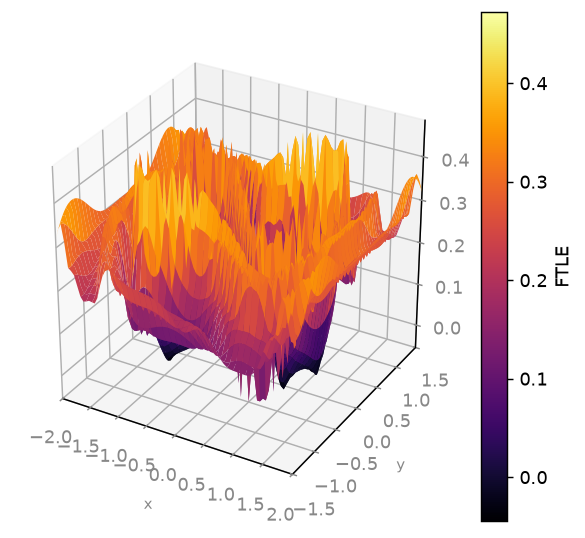
g = ts.viz.geometry(subject, "ftle", grid=201)   # the arrays, and stop there
ts.viz.draw(g, "contour")                        # hand them back to the library
And ts.viz.compatibility() prints the same matrix this page draws.
There are 39 plot transforms and 101 declared (transform, primitive) pairs below. Every figure on this page was produced by the code printed beside it, and the page itself is generated from registry.plot_transforms at build time — so a transform that stopped drawing would take the docs build down with it.
| transform | source | space | primitives (bold = default) | what it draws |
|---|---|---|---|---|
time_series |
data | time |
line, points, steps |
One curve per selected component against time. |
phase_portrait |
data | state2/state3 |
density, line, line3d, points, points3d |
An orbit in state space over an arbitrary component pair or triple. |
delay_embedding |
data | state2 |
density, line, points |
The x(t) vs x(t - delay) reconstruction of a scalar observable. |
phase_portrait_field |
model | state2 |
quiver |
A direction field with a host orbit drawn on it. |
cobweb |
data | state2 |
line, points |
The 1-D staircase x_{n+1} vs x_n with the y = x diagonal. |
spacetime |
data | grid2 |
contour, image, surface3d |
Component index versus time as a colour-mapped lattice. |
spatial_field |
data | grid2 |
contour, image, line, points, surface3d |
A spatially-extended system's field, with the per-time stack for a movie. |
ftle |
model | state2 |
contour, image, surface3d |
The finite-time Lyapunov exponent field; its ridges are the LCS. |
escape_time |
model | state2 |
contour, image, surface3d |
How long each initial condition takes to leave the region. |
transient_time |
model | state2 |
contour, image, surface3d |
How long each initial condition takes to settle onto its attractor. |
invariant_density |
data | scaling/state2 |
contour, histogram, image, line, steps, surface3d |
The natural measure of an orbit: a density curve, or a 2-D measure image. |
psd |
data | scaling |
line, points |
Power spectral density S(f) of one trajectory component. |
autocorrelation |
data | scaling |
line, points, steps |
The autocorrelation C(tau) with its 1/e and first-zero crossings marked. |
mutual_information |
data | scaling |
line, points, steps |
Time-delayed mutual information I(tau) with the chosen delay marked. |
fnn |
data | scaling |
line, points, steps |
Kennel's false-nearest-neighbour fraction against embedding dimension. |
cao |
data | scaling |
line, points, steps |
Cao's averaged-false-neighbour E1(d) / E2(d) against embedding dimension. |
line_lengths |
data | scaling |
line, points, steps |
P(l) and P(v) — the recurrence line-length distributions DET/LAM are read from. |
return_time |
data | scaling |
line, points, steps |
The first-return / first-passage time distribution of a level set. |
hilbert |
data | grid2 |
image, surface3d |
A 1-D observable laid on a space-filling curve as a 2-D image. |
hilbert_fourier |
data | grid2 |
contour, image, surface3d |
The centred 2-D power spectrum of a Hilbert plot — periodicity as symmetry. |
hilbert_difference |
data | grid2 |
contour, image, surface3d |
The locality-loss field — where the curve's 2-D neighbourhood is not a 1-D one. |
hilbert_labels |
data | grid2 |
image |
The curve's own path — each cell coloured by the step at which it is visited. |
nullclines |
model | state2 |
line, points |
The curves f_i = 0 on a 2-D slice; their crossings are the equilibria. |
vector_field |
model | state2 |
quiver |
The right-hand side as arrows on a lattice; unit-length by default. |
flow_speed |
model | state2 |
contour, image, surface3d |
The speed |
streamlines |
model | state2 |
line, points |
Integral curves of the sliced field, seeded on a lattice. |
trace_determinant |
model | param2 |
points |
A system's equilibria placed on the (tr J, det J) stability plane. |
recurrence |
data | grid2 |
contour, image |
The recurrence plot R(i, j) — where the orbit revisits its own neighbourhood. |
poincare_section |
model | state2 |
density, points |
Where an orbit pierces a plane — the flow's discrete portrait. |
orbit_diagram |
model | param1 |
density, points |
The asymptotic orbit against a swept parameter — the bifurcation cascade. |
basins |
model | state2 |
boundary, contour, image |
Which attractor each initial condition reaches — the basin label image. |
ensemble_fan |
data | time |
band |
An ensemble's median with its spread as a shaded envelope. |
lyapunov_spectrum |
data | index |
bars, line, points |
The ordered exponents as a stem plot against the lambda = 0 line. |
lyapunov_convergence |
data | scaling |
line, points |
Each exponent's running Benettin estimate against time — has it settled? |
gali_curves |
data | scaling |
line, points |
GALI_k against time on log axes, with the analytic power-law reference. |
zero_one_pq_plane |
data | state2 |
density, line, points |
The (p, q) translation plane of the 0-1 test: bounded blob or Brownian sprawl. |
scaling_fit |
data | scaling |
line, points |
A log-log scaling curve with the fitted window delimited (+ residual views). |
eigenvalue_plane |
model | complex |
line, points |
The Jacobian spectrum of an equilibrium against its stability boundary. |
floquet_multipliers |
model | complex |
line, points |
A periodic orbit's monodromy spectrum on the unit circle, trivial one marked. |
Data-capable transforms
Computable from a series or a point set — a Trajectory, a bare NumPy array, an analysis result. They also accept a system, because a model gives you data for free (it is integrated once, and the choice is recorded in meta).
time_series
data · time · 3 primitives
One curve per selected component against time.
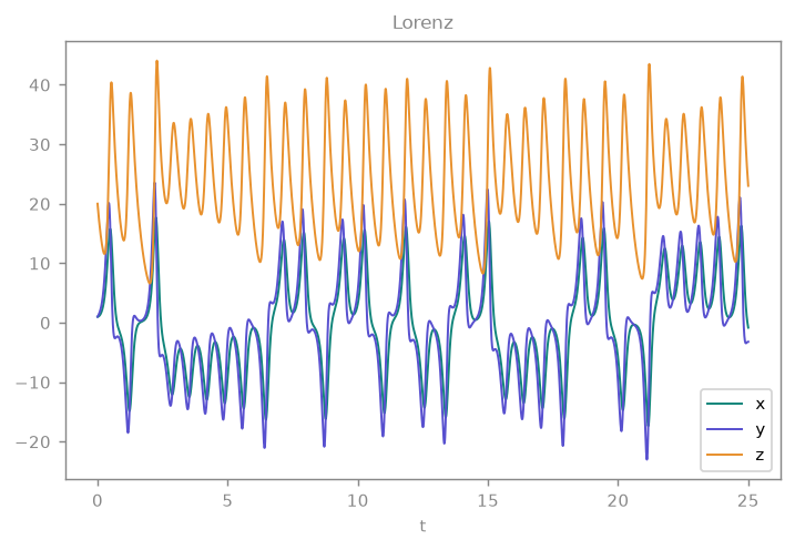
The three Lorenz coordinates against time — one layer per component, coloured from the theme palette. x and y swap sign together at every lobe change; z never goes negative.
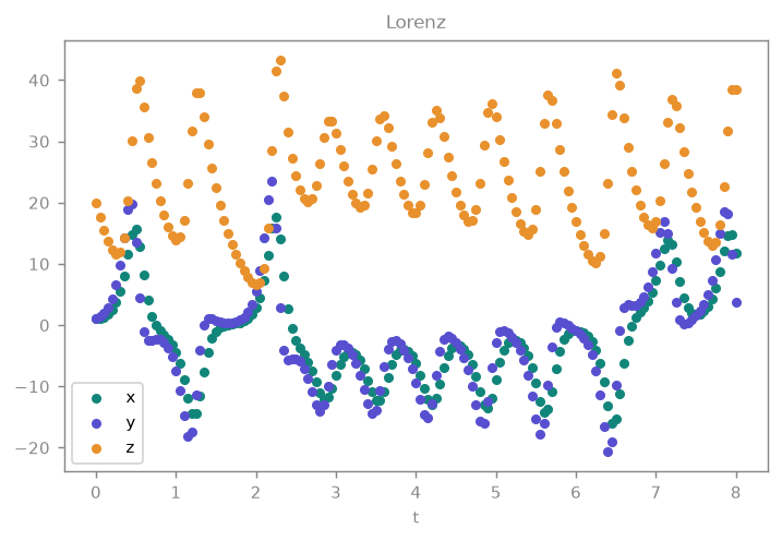
The same series as a scatter — the sampling grid made visible.
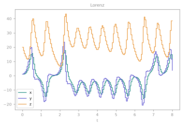
phase_portrait
data · state2/state3 · 5 primitives
An orbit in state space over an arbitrary component pair or triple.
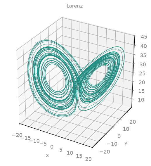
The Lorenz butterfly. With three components selected the geometry is 3-D, so the geometry's own default (line3d) wins over the transform's declared default — which is why asking for flat line here raises instead of silently projecting.
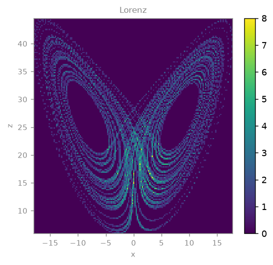
The same projection as a 2-D histogram — where the orbit spends its time, which a line plot hides once the curve overdraws itself. The rims of both wings are where it lingers.
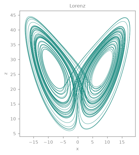
The classic (x, z) projection of the butterfly.
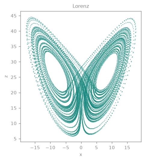
The Lorenz butterfly. With three components selected the geometry is 3-D, so the geometry's own default (line3d) wins over the transform's declared default — which is why asking for flat line here raises instead of silently projecting.
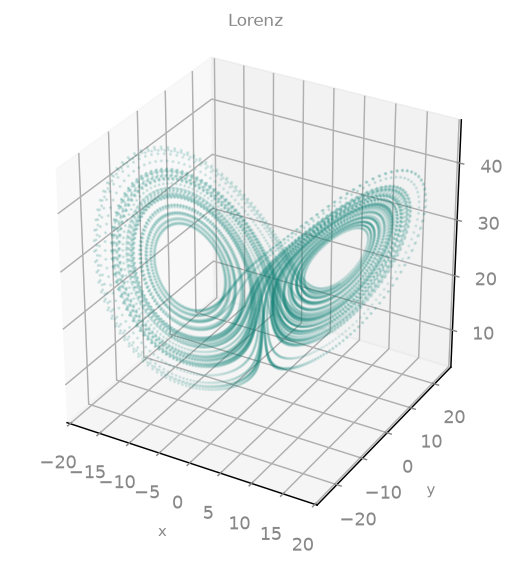
The same orbit as a point cloud — sample density, not connectivity. The style keywords are split out of the same call and applied to this transform's layers.
delay_embedding
data · state2 · 3 primitives
The x(t) vs x(t - delay) reconstruction of a scalar observable.
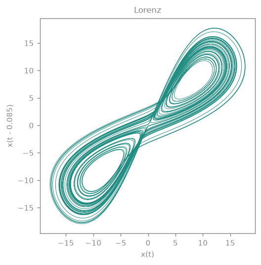
Takens' reconstruction from the single observable x(t): plot it against x(t - τ) and the butterfly reappears, without ever using y or z.
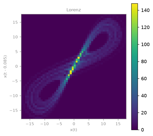
The reconstruction as an occupancy density.
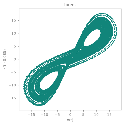
Takens' reconstruction from the single observable x(t): plot it against x(t - τ) and the butterfly reappears, without ever using y or z.
cobweb
data · state2 · 2 primitives
The 1-D staircase x_{n+1} vs x_n with the y = x diagonal.
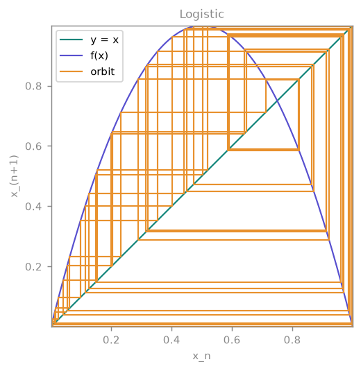
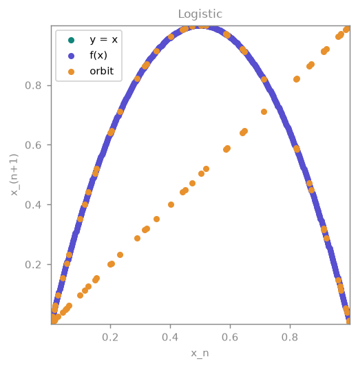
The logistic map at r = 4, iterated as a staircase between the map's graph and the diagonal y = x. Every vertical segment is an application of f, every horizontal one is feeding the result back in. Forty-eight iterates is a cobweb; twenty thousand is a filled square, which is why this one is short on purpose.
spacetime
data · grid2 · 3 primitives
Component index versus time as a colour-mapped lattice.
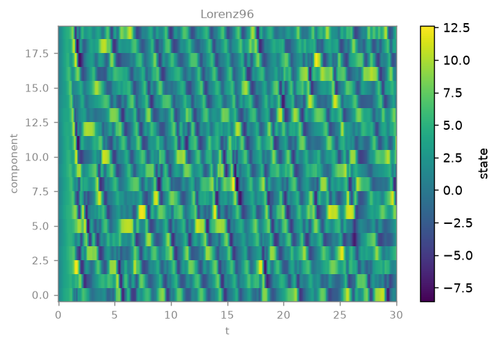
Lorenz-96 as component index versus time: 20 coupled sites, with the westward-drifting waves that a 20-line time series cannot show.
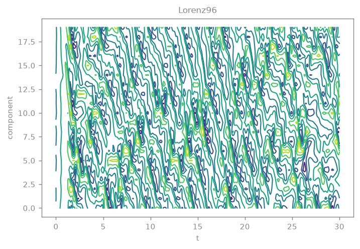
The same lattice as level sets, coloured by level from the transform's colormap rather than by layer index.
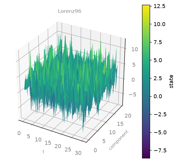
spatial_field
data · grid2 · 5 primitives
A spatially-extended system's field, with the per-time stack for a movie.
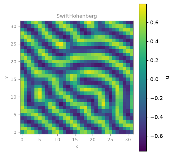
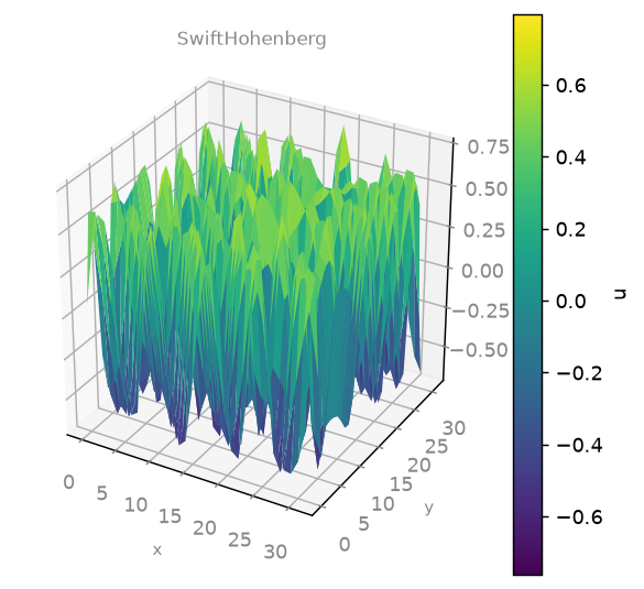
The Swift–Hohenberg field on its own 32×32 grid — the state vector un-flattened by the system's _field_shape, which is why no shape= argument is needed. The stripes are the pattern-forming instability.
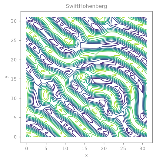
The same field as contours.
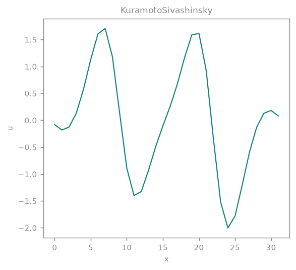
A 1-D field is a profile, not an image: the final Kuramoto–Sivashinsky wave u(x). One transform, two spatial dimensionalities, no guessing.
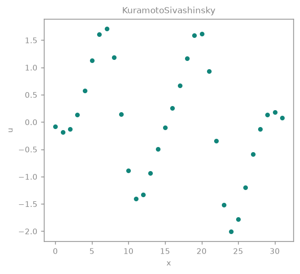
The same profile as its sampled lattice points.
invariant_density
data · scaling/state2 · 6 primitives
The natural measure of an orbit: a density curve, or a 2-D measure image.
Adapts tsdynamics.analysis.planar.invariant_density — the transform itself owns no new math.
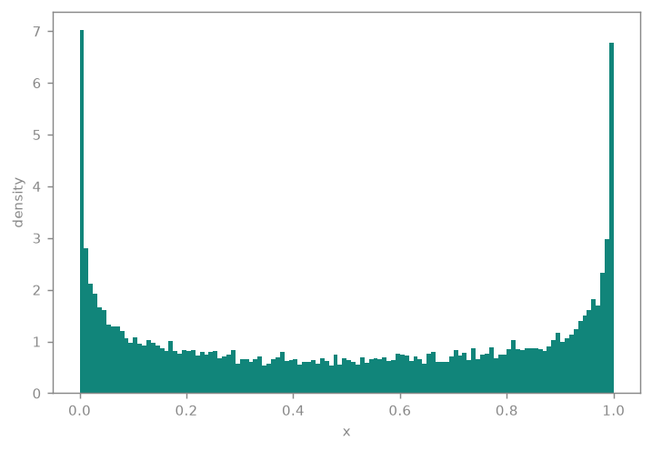
The natural measure of the logistic map at r = 4 — the analytic arcsine law 1/(π√(x(1-x))), with its two integrable spikes at the interval ends, recovered from 20 000 iterates.
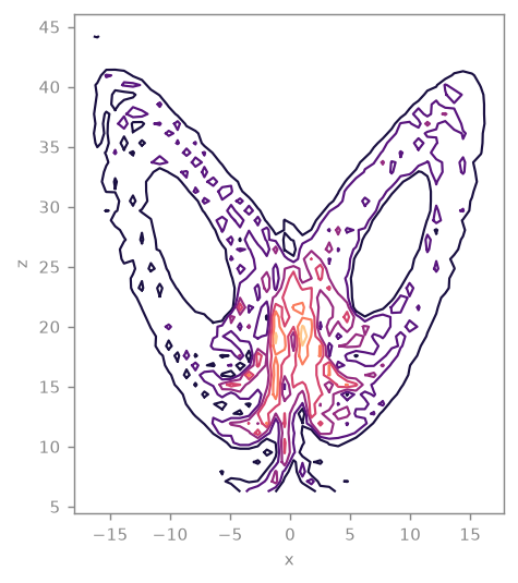
The same 2-D measure as level sets. A histogram needs coarse bins before its level sets mean anything — at 200 bins the contours trace shot noise.
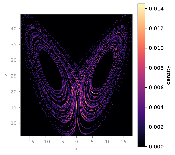
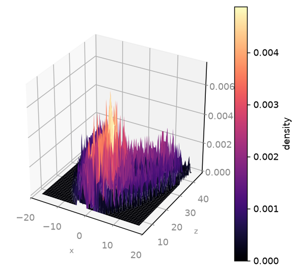
In two components the measure is an image: the Lorenz attractor's occupancy, brightest along the slow spiralling rims.
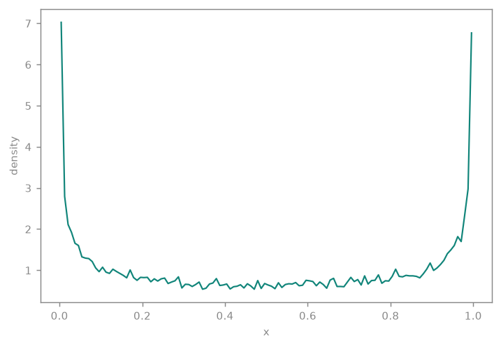
The same density as a curve.
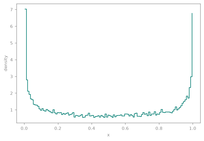
The same density as a step histogram outline.
psd
data · scaling · 2 primitives
Power spectral density S(f) of one trajectory component.
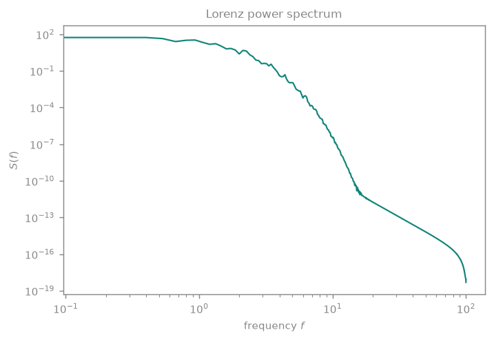
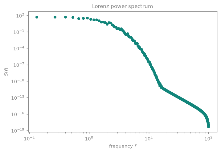
The power spectrum of the Lorenz x coordinate: broadband, a continuum with no line standing out of it — the spectral signature of chaos. The geometry declares log-log axes, because on linear axes every spectrum is a spike at f = 0 and a flat line.
autocorrelation
data · scaling · 3 primitives
The autocorrelation C(tau) with its 1/e and first-zero crossings marked.
Adapts tsdynamics.analysis.embedding.delay.autocorrelation — the transform itself owns no new math.
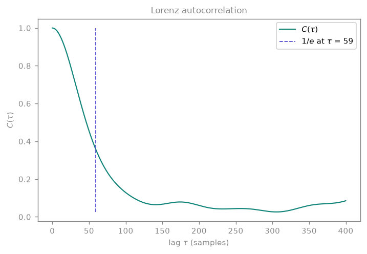
C(τ) for Lorenz x, with the 1/e level and the first zero crossing marked — the two classical rules of thumb for choosing an embedding delay.
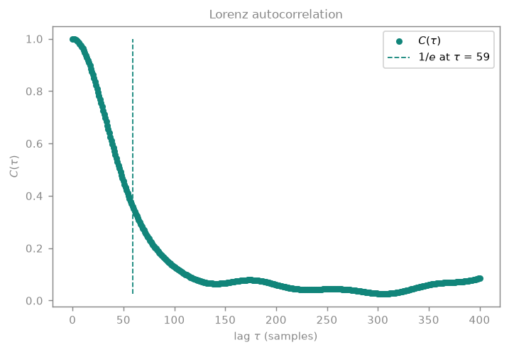
C(τ) for Lorenz x, with the 1/e level and the first zero crossing marked — the two classical rules of thumb for choosing an embedding delay.
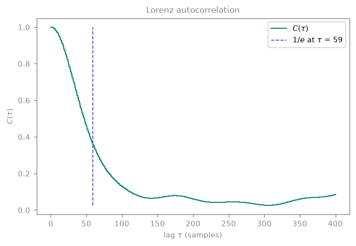
C(τ) for Lorenz x, with the 1/e level and the first zero crossing marked — the two classical rules of thumb for choosing an embedding delay.
mutual_information
data · scaling · 3 primitives
Time-delayed mutual information I(tau) with the chosen delay marked.
Adapts tsdynamics.analysis.embedding.delay.mutual_information — the transform itself owns no new math.
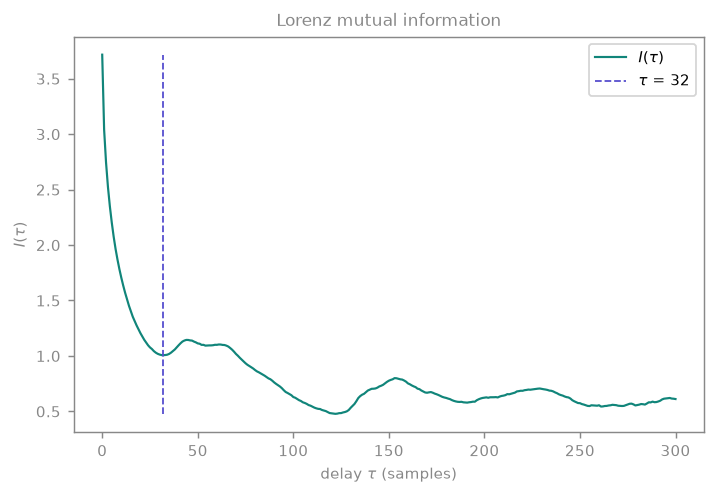
Time-delayed mutual information. Fraser & Swinney's rule takes the first minimum — marked — which is the nonlinear answer to the same question the autocorrelation answers linearly.
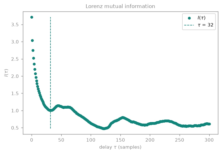
Time-delayed mutual information. Fraser & Swinney's rule takes the first minimum — marked — which is the nonlinear answer to the same question the autocorrelation answers linearly.
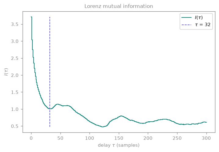
Time-delayed mutual information. Fraser & Swinney's rule takes the first minimum — marked — which is the nonlinear answer to the same question the autocorrelation answers linearly.
fnn
data · scaling · 3 primitives
Kennel's false-nearest-neighbour fraction against embedding dimension.
Adapts tsdynamics.analysis.embedding.dimension.false_nearest_neighbors — the transform itself owns no new math.
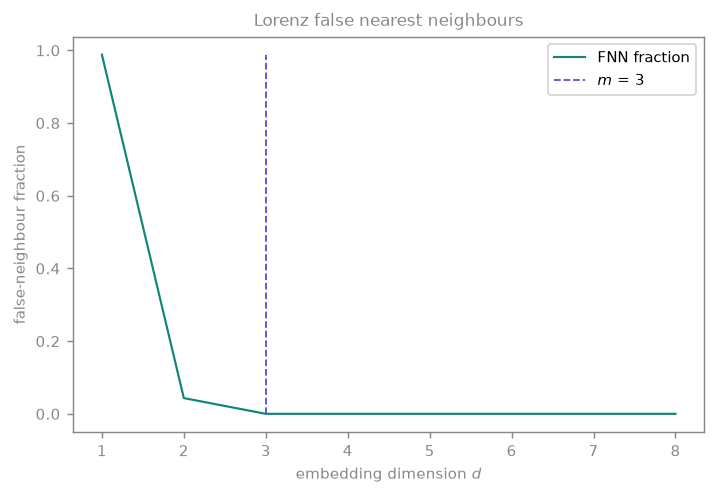
Kennel's false-nearest-neighbour fraction against embedding dimension. It collapses to zero at m = 3 — the true dimension of the Lorenz system, recovered from one scalar observable.
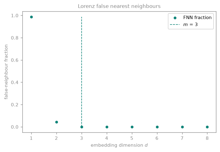
Kennel's false-nearest-neighbour fraction against embedding dimension. It collapses to zero at m = 3 — the true dimension of the Lorenz system, recovered from one scalar observable.
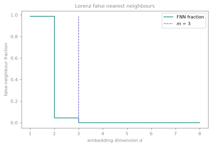
Kennel's false-nearest-neighbour fraction against embedding dimension. It collapses to zero at m = 3 — the true dimension of the Lorenz system, recovered from one scalar observable.
cao
data · scaling · 3 primitives
Cao's averaged-false-neighbour E1(d) / E2(d) against embedding dimension.
Adapts tsdynamics.analysis.embedding.dimension.cao_dimension — the transform itself owns no new math.
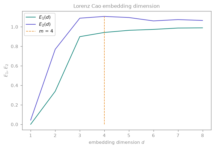
Cao's E1(d) saturates at 1 once the embedding unfolds the attractor, while E2(d) stays away from 1 — which is how the method separates deterministic data from noise, not just picks a dimension.
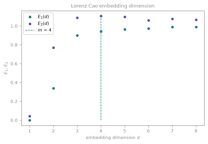
Cao's E1(d) saturates at 1 once the embedding unfolds the attractor, while E2(d) stays away from 1 — which is how the method separates deterministic data from noise, not just picks a dimension.
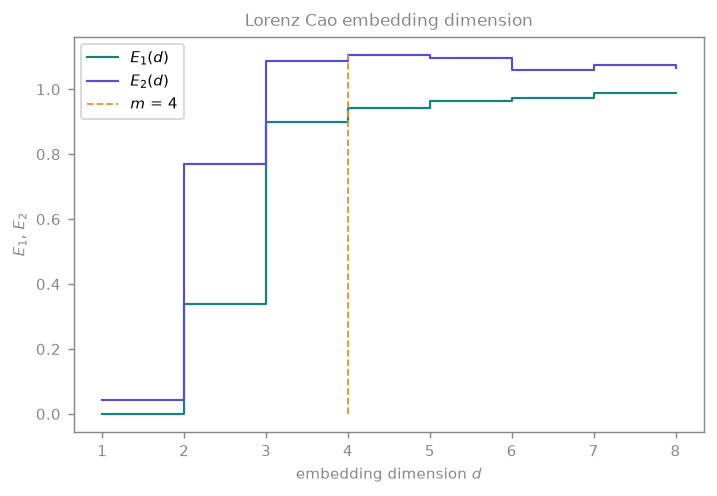
Cao's E1(d) saturates at 1 once the embedding unfolds the attractor, while E2(d) stays away from 1 — which is how the method separates deterministic data from noise, not just picks a dimension.
line_lengths
data · scaling · 3 primitives
P(l) and P(v) — the recurrence line-length distributions DET/LAM are read from.
Adapts tsdynamics.analysis.recurrence.rqa.rqa — the transform itself owns no new math.
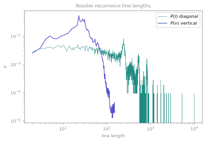
The diagonal and vertical line-length distributions of the recurrence matrix — the histograms that DET, LAM, L_max and TT are read off. Long diagonals mean deterministic recurrence; long verticals mean laminar trapping. Both are heavy-tailed, so they are read on log axes; ts.plot returns the spec, so the fluent tweak chains straight onto the call.
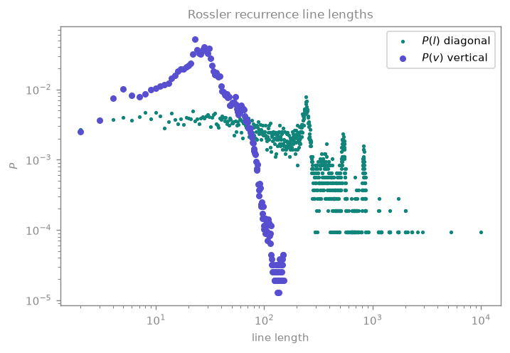
The diagonal and vertical line-length distributions of the recurrence matrix — the histograms that DET, LAM, L_max and TT are read off. Long diagonals mean deterministic recurrence; long verticals mean laminar trapping. Both are heavy-tailed, so they are read on log axes; ts.plot returns the spec, so the fluent tweak chains straight onto the call.
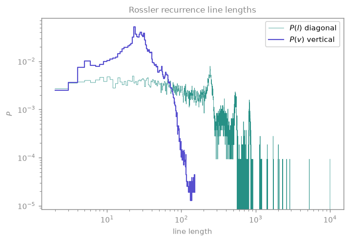
The diagonal and vertical line-length distributions of the recurrence matrix — the histograms that DET, LAM, L_max and TT are read off. Long diagonals mean deterministic recurrence; long verticals mean laminar trapping. Both are heavy-tailed, so they are read on log axes; ts.plot returns the spec, so the fluent tweak chains straight onto the call.
return_time
data · scaling · 3 primitives
The first-return / first-passage time distribution of a level set.
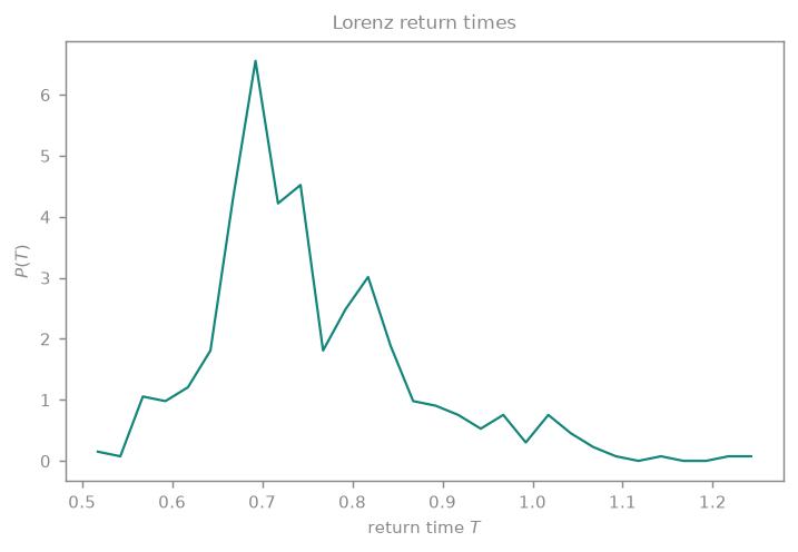
How long the Lorenz orbit takes to come back to a level set of z — one circuit of a wing. The distribution is sharply peaked at T ≈ 0.69 with a right tail: most loops are the same size, and the long ones are the wide swings that follow a lobe change. A periodic orbit would put every count in a single bin; the width of this peak is the chaos.
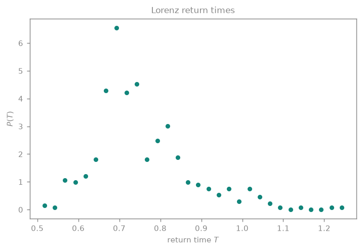
How long the Lorenz orbit takes to come back to a level set of z — one circuit of a wing. The distribution is sharply peaked at T ≈ 0.69 with a right tail: most loops are the same size, and the long ones are the wide swings that follow a lobe change. A periodic orbit would put every count in a single bin; the width of this peak is the chaos.
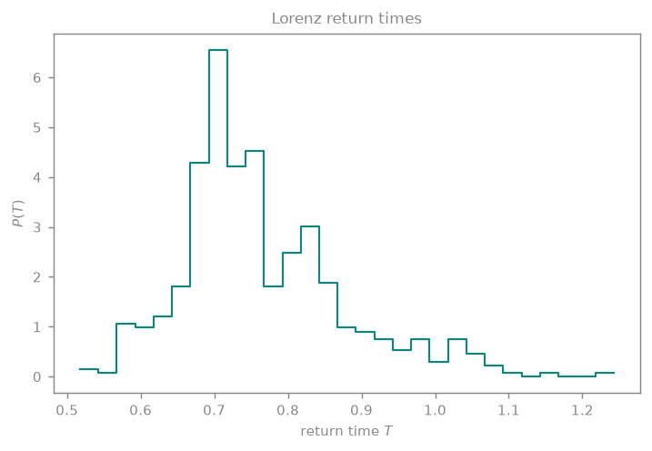
How long the Lorenz orbit takes to come back to a level set of z — one circuit of a wing. The distribution is sharply peaked at T ≈ 0.69 with a right tail: most loops are the same size, and the long ones are the wide swings that follow a lobe change. A periodic orbit would put every count in a single bin; the width of this peak is the chaos.
hilbert
data · grid2 · 2 primitives
A 1-D observable laid on a space-filling curve as a 2-D image.
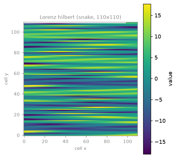
The same record on the dependency-free snake ordering. The Hilbert-type curves need the optional hilbertplot package, which this build does not have; asking for one raises rather than substituting, so what you see is what was asked for.
optional dependency missing — fallback example
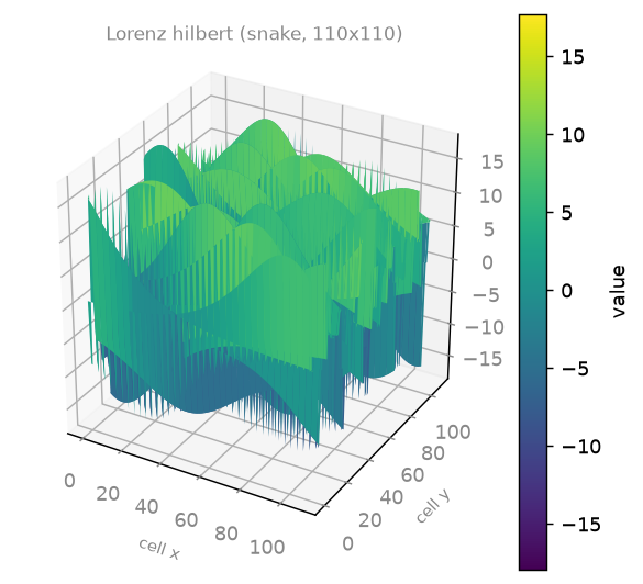
The same record on the dependency-free snake ordering. The Hilbert-type curves need the optional hilbertplot package, which this build does not have; asking for one raises rather than substituting, so what you see is what was asked for.
optional dependency missing — fallback example
hilbert_fourier
data · grid2 · 3 primitives
The centred 2-D power spectrum of a Hilbert plot — periodicity as symmetry.
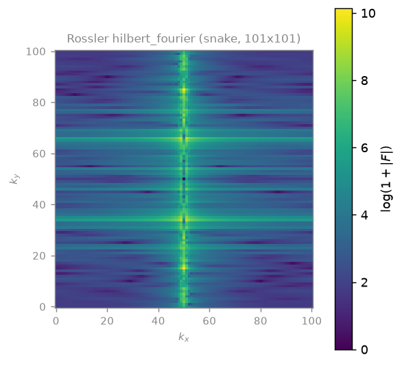
The snake-ordering spectrum — the hilbertplot extra is not installed on this build.
optional dependency missing — fallback example
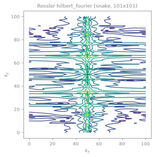
The snake-ordering spectrum — the hilbertplot extra is not installed on this build.
optional dependency missing — fallback example
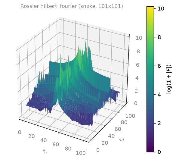
The snake-ordering spectrum — the hilbertplot extra is not installed on this build.
optional dependency missing — fallback example
hilbert_difference
data · grid2 · 3 primitives
The locality-loss field — where the curve's 2-D neighbourhood is not a 1-D one.
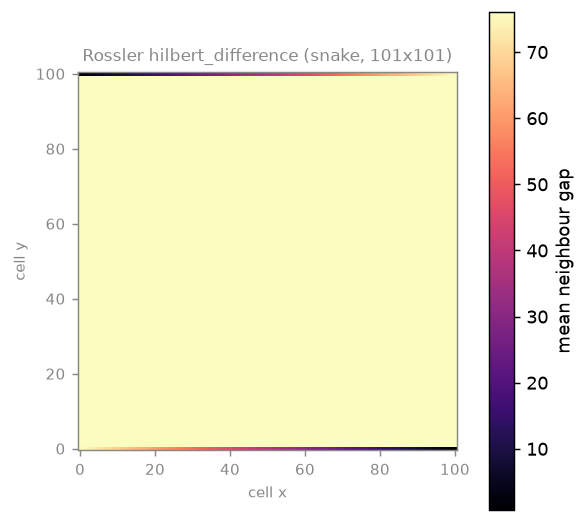
Locality loss for the snake ordering, and it is loss almost everywhere: two vertically adjacent cells are a whole row apart in the record, so the mean neighbour gap is uniformly large — which is exactly the argument for the Hilbert curve, and why this plot is worth having. The hilbertplot extra is not installed on this build, and the transform raises rather than substituting a curve you did not ask for.
optional dependency missing — fallback example
Locality loss for the snake ordering, and it is loss almost everywhere: two vertically adjacent cells are a whole row apart in the record, so the mean neighbour gap is uniformly large — which is exactly the argument for the Hilbert curve, and why this plot is worth having. The hilbertplot extra is not installed on this build, and the transform raises rather than substituting a curve you did not ask for.
optional dependency missing — fallback example
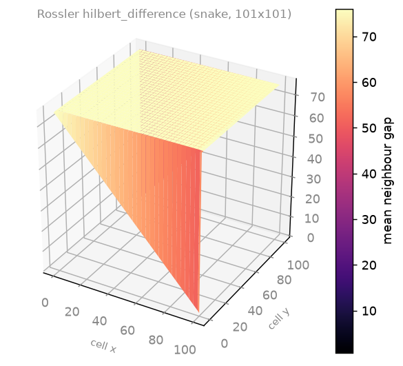
Locality loss for the snake ordering, and it is loss almost everywhere: two vertically adjacent cells are a whole row apart in the record, so the mean neighbour gap is uniformly large — which is exactly the argument for the Hilbert curve, and why this plot is worth having. The hilbertplot extra is not installed on this build, and the transform raises rather than substituting a curve you did not ask for.
optional dependency missing — fallback example
hilbert_labels
data · grid2 · 1 primitive
The curve's own path — each cell coloured by the step at which it is visited.
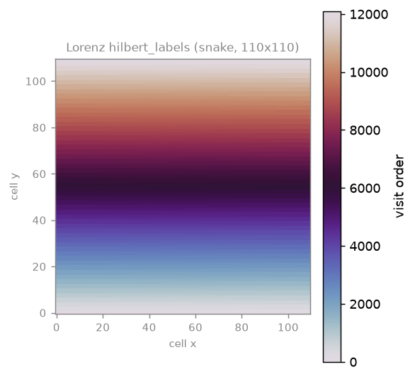
The snake ordering's path: left to right, then right to left. Compare it with the Hilbert curve's recursive quadrant walk to see why locality differs. The hilbertplot extra is not installed here.
optional dependency missing — fallback example
recurrence
data · grid2 · 2 primitives
The recurrence plot R(i, j) — where the orbit revisits its own neighbourhood.
Adapts tsdynamics.analysis.recurrence_matrix — the transform itself owns no new math.
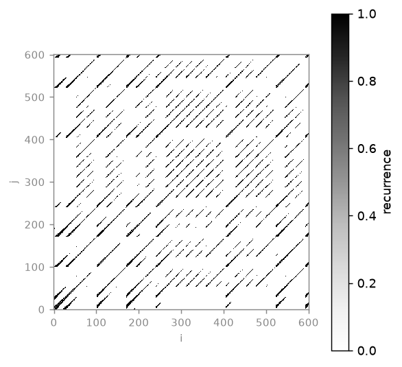
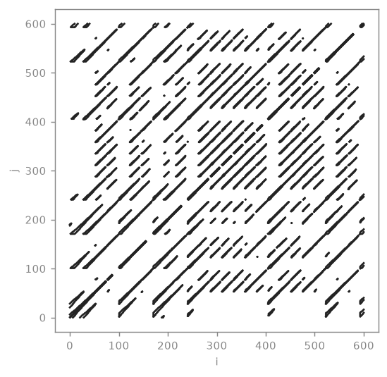
The recurrence plot R(i, j): a dot wherever the orbit returns to within epsilon of an earlier state. The diagonal stripes are near-repetitions of the Rössler cycle; their lengths are what rqa turns into DET and L_max.
ensemble_fan
data · time · 1 primitive
An ensemble's median with its spread as a shaded envelope.
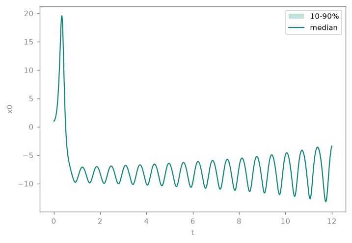
Forty Lorenz starts within 0.05 of each other, drawn as their median and spread. The band is invisible at first and then opens out — sensitive dependence, as a picture of an ensemble rather than of two orbits.
lyapunov_spectrum
data · index · 3 primitives
The ordered exponents as a stem plot against the lambda = 0 line.
Adapts tsdynamics.analysis.lyapunov.lyapunov_spectrum — the transform itself owns no new math.
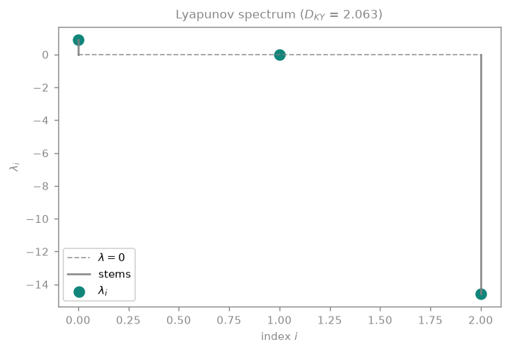
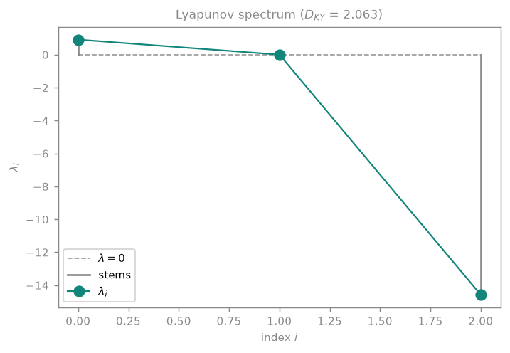
The Lorenz spectrum as a stem plot against the λ = 0 line: one positive exponent (chaos), one zero (the flow direction), one strongly negative (volume contraction). Their sum is the divergence, -(σ + 1 + β).
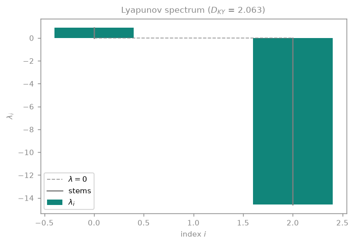
The Lorenz spectrum as a stem plot against the λ = 0 line: one positive exponent (chaos), one zero (the flow direction), one strongly negative (volume contraction). Their sum is the divergence, -(σ + 1 + β).
lyapunov_convergence
data · scaling · 2 primitives
Each exponent's running Benettin estimate against time — has it settled?
Adapts tsdynamics.derived.tangent.TangentSystem.convergence — the transform itself owns no new math.
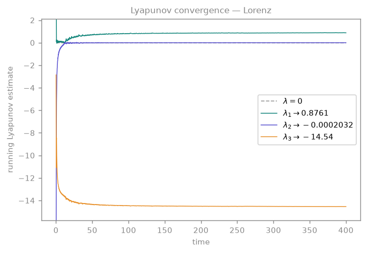
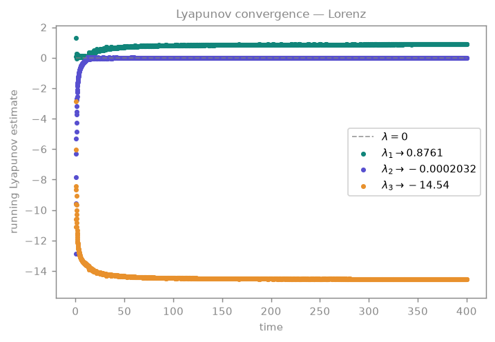
Each exponent's running Benettin estimate against time — the plot that answers has it converged?, which a single returned number never can.
gali_curves
data · scaling · 2 primitives
GALI_k against time on log axes, with the analytic power-law reference.
Adapts tsdynamics.analysis.chaos.gali — the transform itself owns no new math.
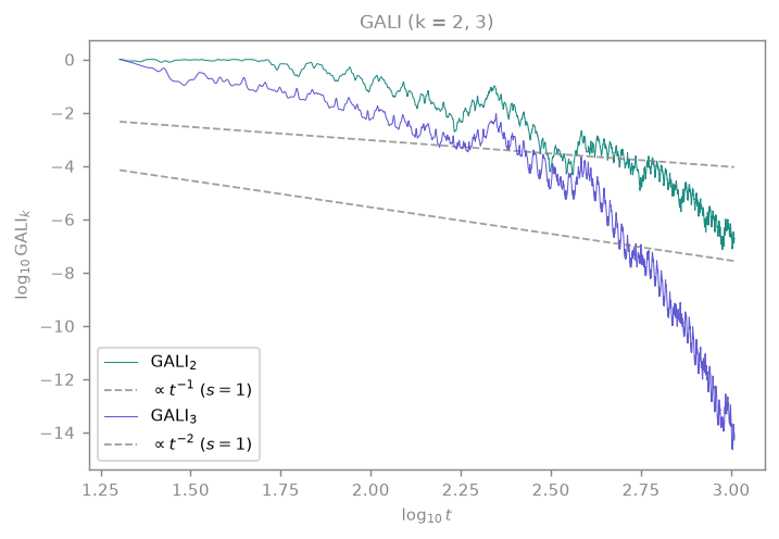
GALI₂ and GALI₃ on log axes for a chaotic Hénon–Heiles orbit, against the analytic reference slope -(k-1)λ₁. Exponential decay is the chaos verdict; a regular orbit would leave GALI₂ flat.
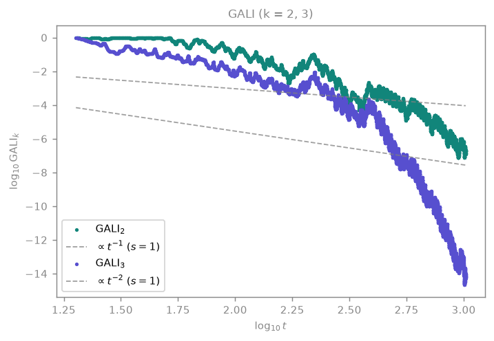
GALI₂ and GALI₃ on log axes for a chaotic Hénon–Heiles orbit, against the analytic reference slope -(k-1)λ₁. Exponential decay is the chaos verdict; a regular orbit would leave GALI₂ flat.
zero_one_pq_plane
data · state2 · 3 primitives
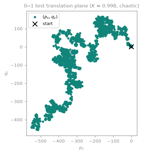
The (p, q) translation plane of the 0-1 test: bounded blob or Brownian sprawl.
Adapts tsdynamics.analysis.chaos.zero_one_test — the transform itself owns no new math.
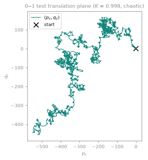
The (p, q) translation variables of the 0–1 test. Chaotic dynamics drives them on a Brownian sprawl whose extent grows without bound; a regular orbit keeps them on a bounded torus-like blob.
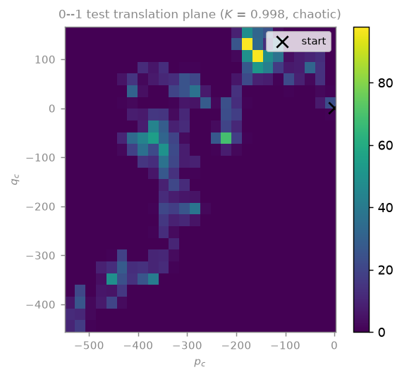
The same walk as an occupancy density.
scaling_fit
data · scaling · 2 primitives
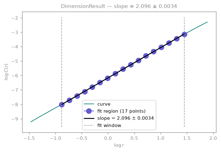
A log-log scaling curve with the fitted window delimited (+ residual views).
Adapts tsdynamics.analysis._result_scaling.ScalingResult — the transform itself owns no new math.
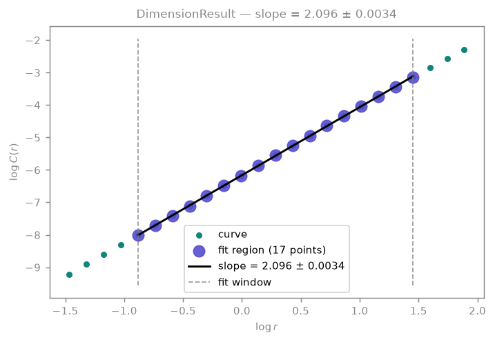
The log-log correlation sum with the fitted scaling window delimited. The slope inside the window is the correlation dimension; the point of drawing it is that you can see whether the window was the right one.
Model-only transforms
These must evaluate or integrate the right-hand side at points that are not in the input, so they need the system itself. Handing one a bare array cannot work, and it says so rather than guessing.
phase_portrait_field
model · state2 · 1 primitive
A direction field with a host orbit drawn on it.
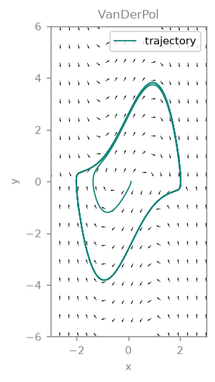
A direction field with its host orbit drawn on it — the orbit is pinned to a line even though the transform's primitive is quiver, because a part may pin its own primitive.
import tsdynamics as ts

import numpy as np

def rhs(u):
    return np.stack([u[..., 1], 2.0 * (1 - u[..., 0] ** 2) * u[..., 1] - u[..., 0]], axis=-1)

traj = ts.systems.VanDerPol(mu=2.0).run(final_time=30.0, dt=0.01, ic=[0.1, 0.0])

ts.plot(rhs, "phase_portrait_field", source=traj, xlim=(-3.0, 3.0), ylim=(-6.0, 6.0), grid=18)
ftle
model · state2 · 3 primitives
The finite-time Lyapunov exponent field; its ridges are the LCS.
Adapts tsdynamics.analysis.planar.ftle_field — the transform itself owns no new math.
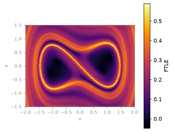
The finite-time Lyapunov exponent field of the unforced two-well Duffing oscillator. The bright ridge is the stable manifold of the saddle at the origin — the separatrix between the two wells, found without ever computing a basin.
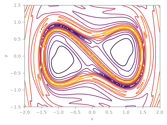
The same field as level sets — the ridge as a contour crowd.
escape_time
model · state2 · 3 primitives
How long each initial condition takes to leave the region.
Adapts tsdynamics.analysis.planar.escape_time_field — the transform itself owns no new math.
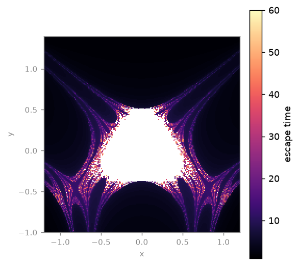
Transient chaos, drawn. Hénon–Heiles above its escape energy: the triangular bound region in the middle (white — never escaped within the horizon, so NaN, a hole rather than a fake number), the three exit channels, and between them the fractal filaments of starts that bounce around for tens of time units before committing to an exit. A two-colour which exit diagram cannot resolve that structure; the level sets of when can. Note at= — the system is 4-D and this is the (x, y) slice at p_y = 0.4, which is what puts it above the escape energy.
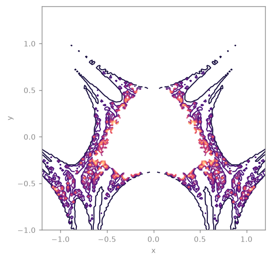
The same field as escape isochrones — a level set is the set of starts that leave the window at the same time.
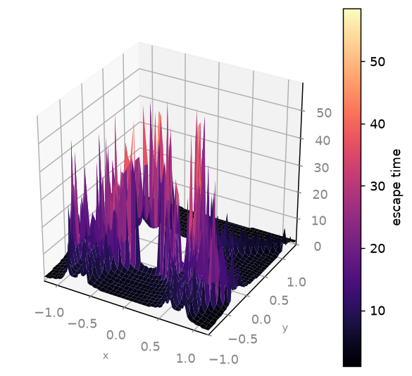
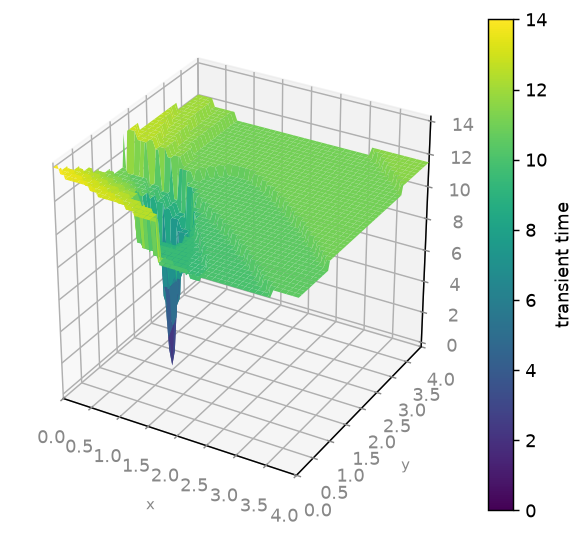
Escape time as a landscape: the spikes are the long-lived orbits on the boundary between exits.
transient_time
model · state2 · 3 primitives
How long each initial condition takes to settle onto its attractor.
Adapts tsdynamics.analysis.planar.transient_time_field — the transform itself owns no new math.
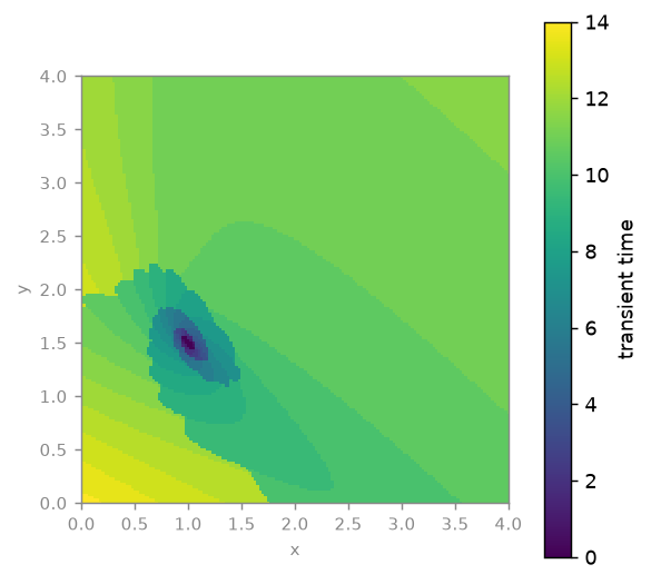
The complement of escape time: how long each start takes to arrive at the Brusselator's stable focus, below its Hopf threshold. The arrival threshold is read off the field itself (1% of the median lattice speed) and recorded in meta, rather than being a fixed number in units the flow has never heard of.
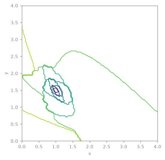
The same field as level sets — each contour is an arrival isochrone.
nullclines
model · state2 · 2 primitives
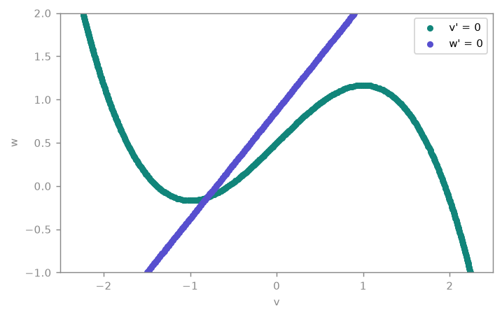
The curves f_i = 0 on a 2-D slice; their crossings are the equilibria.
Adapts tsdynamics.analysis.planar.nullclines — the transform itself owns no new math.
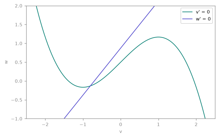
The FitzHugh–Nagumo nullclines: the cubic v' = 0 curve and the straight w' = 0 line. Their crossing is the equilibrium — the textbook picture, computed by marching squares on the real right-hand side.
vector_field
model · state2 · 1 primitive
The right-hand side as arrows on a lattice; unit-length by default.
Adapts tsdynamics.analysis.planar.flow_field — the transform itself owns no new math.
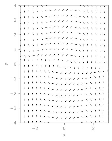
The right-hand side as unit arrows on a lattice — the direction field. Handed the system it infers its own window, exactly as flow_speed does; normalize=False keeps the true magnitudes. direction_field is an alias for this transform, not a second row.
flow_speed
model · state2 · 3 primitives
The speed |f| of the flow as a scalar backdrop.
Adapts tsdynamics.analysis.planar.flow_field — the transform itself owns no new math.
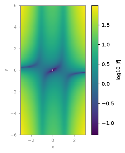
|f| as a backdrop for the Van der Pol relaxation oscillator, on a log scale: the two fast jumps at the ends of the cubic are bright, the two slow crawls along its branches are dark, and the equilibrium at the origin is a hole — log=True maps |f| = 0 to NaN rather than faking a minimum. Speed is exactly what a direction field's unit arrows throw away.
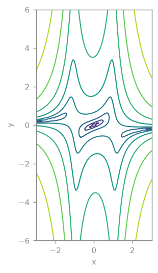
The same speed field as level sets, coloured by level.
streamlines
model · state2 · 2 primitives
Integral curves of the sliced field, seeded on a lattice.
Adapts tsdynamics.analysis.planar.streamlines — the transform itself owns no new math.
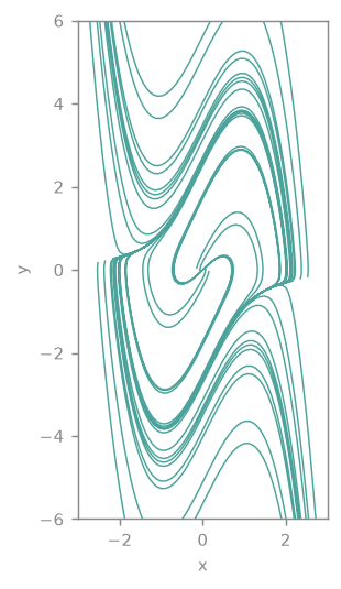
Arc-length-parametrised integral curves of the field, integrated both ways from a lattice of seeds through the system's own right-hand side — not a plotting library's interpolation of a pre-sampled lattice, which is what matters near a separatrix. Every curve is swept onto the same limit cycle, which is the picture of an attractor.
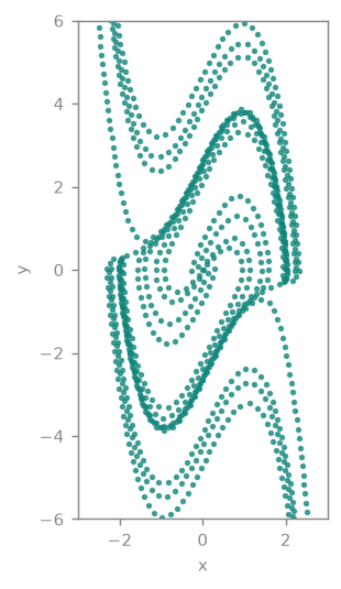
The streamline vertices: evenly spaced by arc length, not by time — so their spacing carries no speed information, deliberately.
trace_determinant
model · param2 · 1 primitive
A system's equilibria placed on the (tr J, det J) stability plane.
Adapts tsdynamics.analysis.planar.trace_determinant — the transform itself owns no new math.
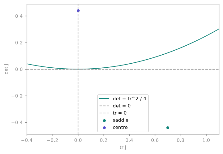
Every equilibrium of the system placed on the (tr J, det J) plane, with the axes and the discriminant parabola that partition it into node / spiral / saddle / centre. Lotka–Volterra's two equilibria land in two different regions: the extinction state below the det = 0 axis is a saddle, the coexistence state on the tr = 0 axis is a centre — which is why its orbits are closed. The frame is param2, so this correctly refuses to overlay on a state space.
poincare_section
model · state2 · 2 primitives
Where an orbit pierces a plane — the flow's discrete portrait.
Adapts tsdynamics.analysis.poincare_section — the transform itself owns no new math.
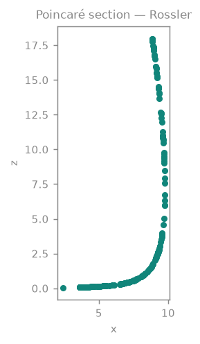
(No curated example yet — drawn on the small fixture poincare_section registers for the compatibility gate. Add one to docs/_tooling/gallery.py.)
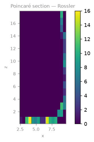
(No curated example yet — drawn on the small fixture poincare_section registers for the compatibility gate. Add one to docs/_tooling/gallery.py.)
orbit_diagram
model · param1 · 2 primitives
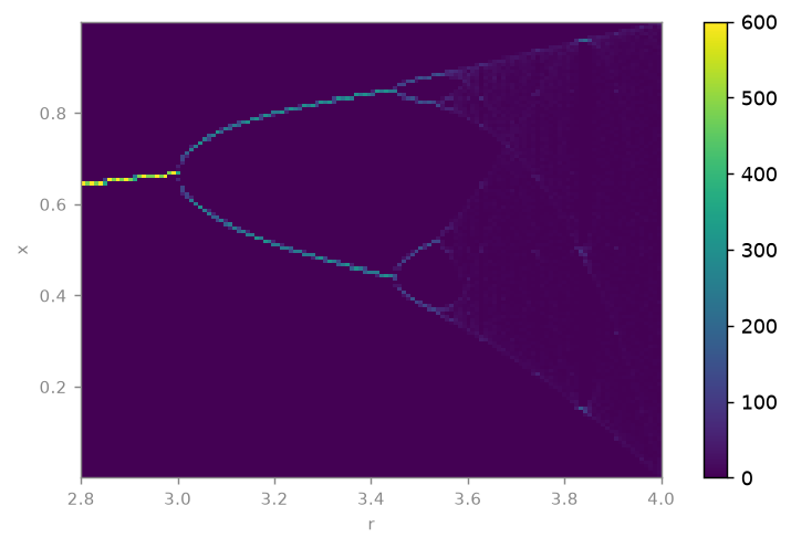
The asymptotic orbit against a swept parameter — the bifurcation cascade.
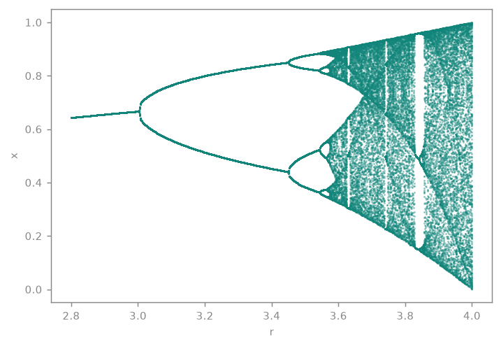
The period-doubling cascade, drawn as a transform rather than read off a result — so it overlays, grids and styles like any other layer. One fixed point doubles at r = 3, again at 1 + sqrt(6), and smears into chaos near 3.57, threaded with periodic windows.
basins
model · state2 · 3 primitives
Which attractor each initial condition reaches — the basin label image.
Adapts tsdynamics.analysis.basins — the transform itself owns no new math.
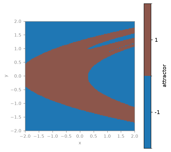
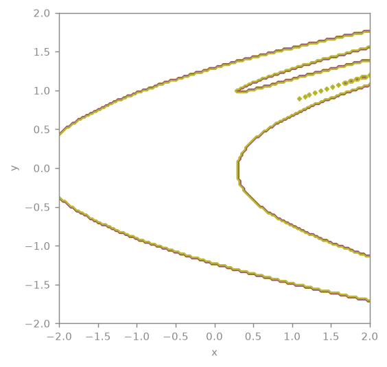
Which fate each initial condition meets: the Hénon attractor's basin against the starts that escape to infinity. The boundary is the stable manifold of the saddle at infinity — smooth here, fractal for many other systems, which is what basin_entropy measures.
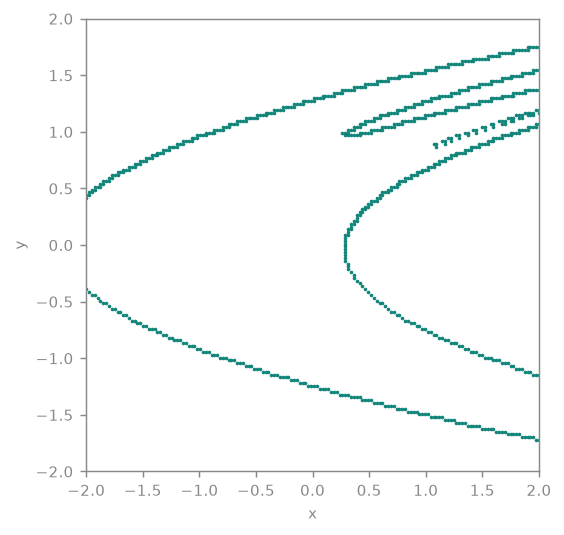
Only the cells on the basin boundary — the set whose fate a small perturbation can change.
eigenvalue_plane
model · complex · 2 primitives
The Jacobian spectrum of an equilibrium against its stability boundary.
Adapts tsdynamics.analysis.fixedpoints.fixed_points — the transform itself owns no new math.
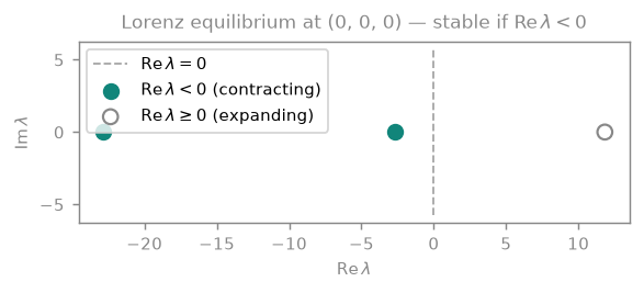
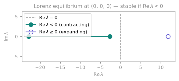
The Jacobian spectrum of the Lorenz origin against the imaginary axis: {+11.83, -2.67, -22.83} — one eigenvalue to the right of the boundary, so the origin is the saddle that separates the two wings. The boundary is real geometry in its own layer, so it survives JSON and three.js export.
floquet_multipliers
model · complex · 2 primitives
A periodic orbit's monodromy spectrum on the unit circle, trivial one marked.
Adapts tsdynamics.analysis.fixedpoints.periodic_orbit — the transform itself owns no new math.
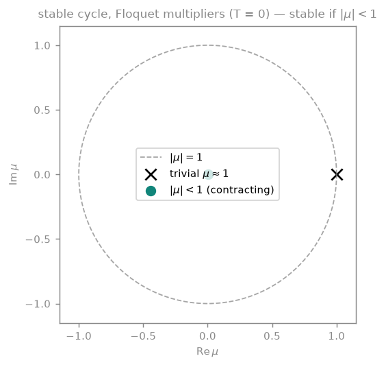
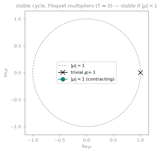
The monodromy spectrum of the Van der Pol limit cycle (period T = 6.663) against the unit circle. One multiplier sits at +1 — the trivial one, along the flow, found by aligning the eigenvector with f(x₀) and marked as such. The other is at the origin to plotting accuracy (|μ| ~ 1e-3), which is what strongly attracting means.
Compositions
Nothing above is a special case: a transform's geometry declares the coordinate space it lives in, and any two that agree can share one set of axes. That is what makes the overlays below one call rather than a figure-assembly exercise — and it is also why an (x, z) portrait refuses (x, y) equilibria, and why the (tr J, det J) plane refuses a state space:
InvalidParameterError: cannot overlay frame 'param2' (diagnostic_curve) on frame 'state2'
(phase_portrait_2d): they are drawings of different spaces. Use layout='stack' / 'row' / 'grid'
to give each its own panel.
The phase-plane payoff
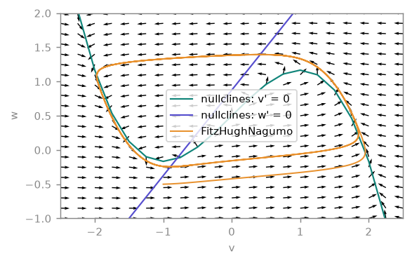
Four things on one axes, from three different transform families: the direction field, both nullclines, and an integrated orbit. The equilibrium is where the nullclines cross, the orbit is tangent to the arrows everywhere, and the relaxation loop rides the outer branches of the cubic. Draw order is by role — field under curve — so the arguments could be given in any order.
import tsdynamics as ts

fhn = ts.systems.FitzHughNagumo()
traj = fhn.run(final_time=120.0, dt=0.05, ic=[-1.0, -0.5])

ts.viz.plot(
    ts.plot(fhn, "direction_field", "nullclines",
            xlim=(-2.5, 2.5), ylim=(-1.0, 2.0), grid=21),
    ts.plot(traj, "phase_portrait"),
)
Speed under streamlines
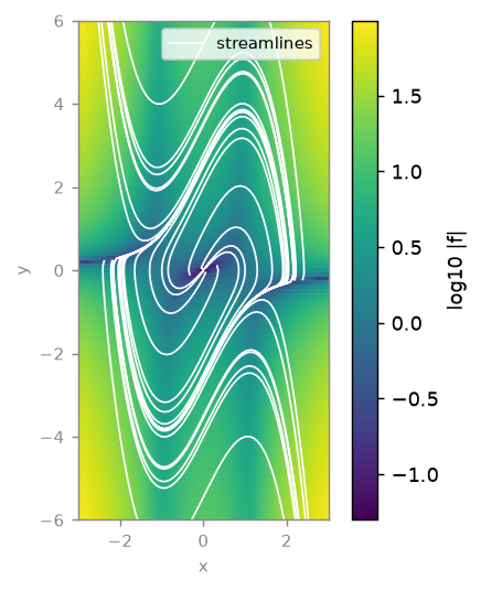
One call, two model transforms, one shared window: the speed field as the backdrop and its integral curves on top. A shared keyword is routed only to the transforms that accept it — log= reaches flow_speed, seeds= reaches streamlines, and neither gets the other's.
import tsdynamics as ts

vdp = ts.systems.VanDerPol(mu=2.0)

ts.plot(vdp, "flow_speed", "streamlines",
        xlim=(-3.0, 3.0), ylim=(-6.0, 6.0), log=True, seeds=5, steps=120)
A separatrix, twice
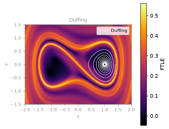
An orbit drawn on the FTLE field of its own system. The orbit spirals inside one well and never crosses the bright ridge — which is the claim the ridge makes: it is the separatrix, computed from the variational dynamics, not from watching where orbits end up.
import tsdynamics as ts

duff = ts.systems.Duffing(gamma=0.0)
traj = duff.run(final_time=60.0, dt=0.01, ic=[1.4, 0.0, 0.0])

ts.viz.plot(
    ts.plot(duff, "ftle", xlim=(-2.0, 2.0), ylim=(-1.5, 1.5),
            grid=161, final_time=8.0),
    ts.plot(traj, "phase_portrait", components=("x", "y"), color="w"),
)
Adding a plot
A new transform is one registration and nothing else — no renderer edit, no
PlotKind edit, no compose edit, no test edit:
Four declarations and a function that returns a mapping. Nothing else in the library is edited:
# skip-doctest — a template: `measure` is yours, and registering a placeholder
# transform here would put it in every listing for the rest of the session
import tsdynamics as ts

@ts.viz.transforms.register(source="data",              # or "model"
                            frame="scaling",
                            kind="scaling_curve",
                            primitives=("line", "points"))
def my_diagnostic(subject, *, option=1.0):
    """One line — it becomes the summary in the matrix above."""
    r, c = measure(subject, option)
    return {"x": r, "y": c}              # a plain channel mapping — no IR type
Everything else is derived: the name from the function, the summary from the
docstring, the axis count from the frame's arity, the default primitive from the
first one listed, the accepted subjects from source. The optional keywords are
name=, default_primitive=, aliases=, labels=, role=, analysis= (the
estimator this adapts) and example= (a small subject the gallery can draw).
The registration carries the compatibility row, so
tests/test_viz_compatibility.py starts rendering every cell of it, and this
gallery starts showing it — on the small fixture the example= factory returns,
until someone curates a nicer subject in docs/_tooling/gallery.py. The
generator prints any uncurated transform at the end of a run, so a new one is
visible the moment it lands.
Out of tree, declare the same function against the tsdynamics.plot_transforms
entry-point group and it joins the registry — and this page — on import.