Analysis · Poincaré sections

Poincaré sections¶

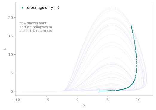
A continuous flow is hard to see: a 3-D attractor is a tangle, a higher-D one is invisible. Poincaré's device is to stop watching the whole trajectory and record only the moments it pierces a chosen surface. That reduces the flow by one dimension and turns it into a discrete map — periodic orbits become finite point sets, a strange attractor becomes fractal dust with visible structure, and the whole quantifier toolkit written for maps suddenly applies to the flow.

The idea¶

Pick a hyperplane \(\Sigma\) in state space and watch the trajectory cross it, always in the same direction. The ordered sequence of crossing points \(\mathbf{u}_0, \mathbf{u}_1, \dots\) is the surface of section, and the rule \(\mathbf{u}_n \mapsto \mathbf{u}_{n+1}\) that carries one crossing to the next is the Poincaré (first-return) map. A period-\(T\) orbit that crosses \(\Sigma\) once per period shows up as a single fixed point of that map; a quasi-periodic torus as a closed loop; a chaotic attractor as a structured cloud of one lower dimension than the flow. The section throws away the flow between crossings but keeps everything that matters for the topology of the attractor.

From a system: root-refined crossings¶

Hand poincare_section a flow and the plane, and it returns the crossings:

import tsdynamics as ts

section = ts.poincare_section(
    ts.systems.Rossler(),
    plane=("y", 0.0, "up"),   # section y = 0, crossed upward
    n=500,
)

section.t          # crossing times, shape (500,)
section.y          # full-dimensional crossing states, (500, 3)
section.summary()  # crossings / dim / plane / direction

The system path marches the flow with a detection step dt, brackets each sign change of the plane function, and refines the crossing with cubic Hermite interpolation — endpoint derivatives come from the system's numeric right-hand side, giving \(O(\Delta t^4)\) accuracy in the crossing point. dt only has to be small enough not to skip a crossing; the refinement supplies the precision.

The return value is a PoincareSection — a Trajectory subclass carrying section plot intent (so a renderer draws the in-plane scatter, not a misleading flow line) plus a .summary() / .to_dict() / .plot result surface.

Rössler flow crossed by the section y = 0 — FIG 1 · the Rössler flow (faint indigo, x–z projection) crossed by the plane y = 0: the teal crossings collapse from the full 2-D-looking attractor onto a thin, near-one-dimensional return set — the hallmark of a Poincaré section.

Under the hood this runs on the wired Rust event engine: the whole attractor is marched and every crossing refined in a single engine call, roughly two orders of magnitude faster than a per-dt Python loop. DDEs (no numeric RHS), stiff defaults, and backend="reference" transparently fall back to the Python loop; the two paths are answer-identical at the same fixed-step discretisation.

From trajectory data: no system needed¶

If you only hold arrays — archived output, an experimental record — pass the Trajectory instead:

traj = ts.systems.Lorenz().integrate(final_time=300.0, dt=0.01)
section = ts.poincare_section(traj, plane=("z", 25.0))   # plane z = 25

The data path finds sign changes between consecutive samples and locates each crossing by linear interpolation. It needs nothing but the arrays, but its accuracy is bounded by the trajectory's sampling interval (\(O(\Delta t^2)\)). When you still hold the system, prefer the system path — it refines to a far tighter tolerance than the grid you happened to save.

Specifying the plane¶

The plane= argument accepts three spellings; the friendly one names a coordinate and a direction word.

Spec	Meaning
`("y", 0.0)` — name + offset	Axis-aligned section \(y = 0\), with `direction=` deciding orientation
`("y", 0.0, "up")` — name + offset + direction	The same, with the crossing direction inline (overrides `direction=`)
`(1, 0.0)` — index + offset	Axis-aligned section on component 1 (indices work when no `variables` are declared)
`([1, 0, 0], 0.0)` — normal + offset	The general section \(\mathbf{n}\cdot\mathbf{y} = \text{offset}\) for an arbitrary normal vector

A component name is resolved against the system's variables; a wrong name or a name on a system without variables raises InvalidParameterError with a hint. The direction words are "up" (increasing through the plane, the default), "down", and "both":

ts.poincare_section(traj, plane=("y", 0.0, "up"))    # only upward crossings
ts.poincare_section(traj, plane=("y", 0.0), direction="down")
ts.poincare_section(traj, plane=("y", 0.0, "both"))  # both orientations

One-sided sections are usually what you want — a two-sided section superimposes the two halves of the attractor and blurs the return structure.

skip_crossings, not transient

To discard leading crossings while the flow settles onto the attractor, use skip_crossings= — a count of crossings, deliberately distinct from the time- or step-based transient of other analyses. The section transient is measured in section hits, so the vocabulary keeps them apart.

The `PoincareMap` wrapper¶

poincare_section is a convenience over the real machinery, the PoincareMap derived system. Because a PoincareMap is a discrete System, it slots into anything written for maps:

from tsdynamics import PoincareMap

pmap = PoincareMap(ts.systems.Rossler(), plane=("y", 0.0, "up"), dt=0.01)

u1 = pmap.step()             # advance the flow to the next crossing
sec = pmap.trajectory(500)   # collect 500 crossings → PoincareSection
pmap.crossing_count          # bookkeeping

The most important consumer is orbit_diagram: a parameter sweep over a PoincareMap is a bifurcation diagram of the flow. PoincareMap also exposes the section to the general events API via pmap.as_events(), so the same crossings can be collected through system.run(events=...). A ConvergenceError is raised if no crossing occurs within max_time — the plane may miss the attractor, or the direction is reversed.

First-return maps¶

A return map takes the reduction one step further: from the crossing sequence it keeps a single scalar observable and plots each value against its successor \((v_n, v_{n+1})\), exposing the one-dimensional map that governs the flow. return_map(method="poincare") builds it directly from a section:

rm = ts.return_map(ts.systems.Rossler(), "y", method="poincare",
                   plane=("x", 0.0, "up"), n=400)

The related extremum construction — successive local maxima of a coordinate, the Lorenz \(z\)-maxima cusp — is covered on the orbit-diagrams page. A tight, single-valued curve means a noisy 1-D map governs the dynamics; a filled cloud means it does not.

References¶

Poincaré, H. (1899). Les méthodes nouvelles de la mécanique céleste. Gauthier-Villars.
Hénon, M. (1982). On the numerical computation of Poincaré maps. Physica D 5, 412–414.
Lorenz, E. N. (1963). Deterministic nonperiodic flow. J. Atmos. Sci. 20, 130–141.