Analysis · Chaos indicators

Chaos indicators¶

Sometimes you do not want the whole Lyapunov spectrum — you want a verdict. Is this orbit chaotic or regular? TSDynamics ships three fast, literature-validated tests that answer it from three different angles: the alignment of tangent vectors, a single scalar drawn from one observable, and the growth of a derivative-volume that estimates topological entropy. Each is cheap, each returns a result you can threshold, and together they cross-check one another.

GALI_2 and GALI_3 for the Lorenz attractor decaying exponentially against their Skokos-law reference slopes on a semilog axis — On the chaotic Lorenz attractor both alignment indices collapse exponentially, and their decay rates are fixed by the Lyapunov gaps: GALI₂ (indigo) falls at $\lambda_1-\lambda_2 \approx 0.91$ (with $\lambda_2 \approx 0$ along the flow), while GALI₃ (teal) falls at $(\lambda_1-\lambda_2)+(\lambda_1-\lambda_3) \approx 16.4$, hitting the floating-point floor almost at once — the measured curves tracking the predicted Skokos-law slopes (dashed).

Function	Reads	Chaotic ⇒	Regular ⇒
`gali`	tangent-vector volume	exponential decay	$\sim O(1)$ / power law
`zero_one_test`	scalar $K \in [-1, 1]$	$K \approx 1$	$K \approx 0$
`expansion_entropy`	$H$ (topological entropy)	$H > 0$	$H \approx 0$

Maps use the compiled analytic Jacobian; flows use a self-contained RK4 variational core. Both are backend-free (the fast tier — no engine compile step), so these tests are cheap to sweep over a parameter or an ensemble.

GALI — Generalized Alignment Index¶

gali evolves $k$ deviation vectors along the orbit and tracks the volume of the parallelepiped they span (Skokos, Bountis & Antonopoulos 2007). Written as a wedge product of the normalised deviation vectors,

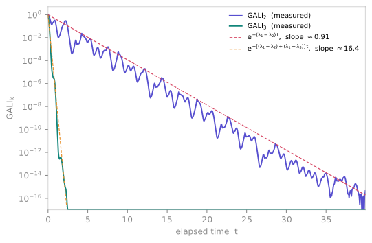
\[ \mathrm{GALI}_k(t) = \lVert \hat w_1(t) \wedge \dots \wedge \hat w_k(t) \rVert = \prod_{i=1}^{k} \sigma_i, \]

it is the product of the singular values $\sigma_i$ of the matrix of deviation vectors. For a chaotic orbit every vector rotates toward the most-expanding direction, so the volume collapses exponentially at a rate set by the leading Lyapunov gaps,

\[ \mathrm{GALI}_k(t) \sim e^{-[(\lambda_1-\lambda_2)+\dots+(\lambda_1-\lambda_k)]\,t}. \]

For regular (quasi-periodic) motion it stays $O(1)$ or decays only by a power law. Crucially the deviation vectors are not re-orthonormalised — only per-column renormalised — which is exactly what lets the spanned volume actually shrink.

import tsdynamics as ts

g = ts.gali(ts.systems.Lorenz(), 2, final_time=40.0, dt=0.05, ic=[1.0, 1.0, 1.0])

g.values[0], g.values[-1]   # ≈ 1.0  →  ~1e-16   (exponential collapse: chaotic)
g.is_chaotic()              # True
g.decay_rate()              # ≈ 0.82  →  λ₁ − λ₂  (the Skokos law; lit. ≈ 0.906)
g.is_discrete               # False

The GALIResult carries the full decay curve — g.k, g.times, g.values, g.is_discrete — and float(g) is the final value, so the result drops straight into a threshold test. g.decay_rate() fits the log-slope over the samples above the numerical floor to recover the exponent-gap sum, and g.is_chaotic() thresholds the final value. Note k is the second positional argument, and must satisfy $2 \le k \le \dim$.

# GALI_3 on Lorenz: the second gap (λ₁ − λ₃ ≈ 15.5) is added on top, so it
# decays far faster — the teal curve in the figure above.
ts.gali(ts.systems.Lorenz(), 3, final_time=40.0, dt=0.05,
        ic=[1.0, 1.0, 1.0]).decay_rate()   # ≈ 18.4  (lit. gap sum ≈ 16.4)

# On a map GALI is immediate (analytic Jacobian, no integration):
ts.gali(ts.systems.Henon(), 2, n=60).is_chaotic()    # True

GALI on a flow integrates its variational core

gali on a map is immediate; on a flow the deviation vectors are advanced by the internal RK4 variational core, so it is slower. The measured decay rate of $\mathrm{GALI}_2$ on Lorenz ($\approx 0.82$ over this short orbit) approximates the Skokos-law gap $\lambda_1 - \lambda_2 \approx 0.906$ (with $\lambda_2 = 0$ along the flow); a short, un-renormalised horizon is a finite-time estimate, so the number brackets rather than nails the exponent gap. See Lyapunov spectra for the spectrum itself.

GALI characterises a specific orbit, so an explicit ic that escapes the basin raises rather than being silently swapped for a random one — pass an ic from a known basin point, or omit it to roll (and, if it diverges, retry) a random one.

The 0–1 test¶

zero_one_test answers the question from a single scalar observable — no phase-space reconstruction, no Jacobian at all (Gottwald & Melbourne 2004, 2009). For each of many random frequencies $c$ it drives a skew translation,

\[ p_c(n) = \sum_{j=1}^{n} \phi_j \cos(jc), \qquad q_c(n) = \sum_{j=1}^{n} \phi_j \sin(jc), \]

and measures the asymptotic growth of the mean-square displacement of $(p_c, q_c)$. Regular dynamics keep the translation bounded (growth $K_c \approx 0$); chaotic dynamics make it diffuse like a random walk (linear growth, $K_c \approx 1$). The returned $K$ is the median of $K_c$ over the frequencies, computed by the regularised correlation method of the 2009 paper.

ts.zero_one_test(ts.systems.Logistic(params={"r": 4.0}), n=5000, ic=[0.1])   # ≈ 0.998  (chaotic)
ts.zero_one_test(ts.systems.Logistic(params={"r": 3.5}), n=5000, ic=[0.1])   # ≈ 0.0    (period-4 window)

The first argument may be a system — integrated (a flow) or iterated (a map / Poincaré / stroboscopic view) internally to produce the observable — or a bare 1-D series read directly (the data overload):

x = ts.systems.Logistic(params={"r": 4.0}).iterate(steps=5000, ic=[0.1]).component("x")
ts.zero_one_test(x)          # ≈ 0.998   (the data overload — horizon keywords don't apply)

The test medians over n_c random drive frequencies drawn from c_range (defaulting to the interval that avoids the resonances near $c = 0, \pi$); pass seed= for a reproducible draw, and return_distribution=True to also get the per-frequency $K_c$ array. The ZeroOneResult is a drop-in for its $K$ value and also carries the translation plane $(p_c, q_c)$ — a bounded blob for regular motion, a diffusing cloud for chaos — which result.plot() renders as a phase portrait.

Noise-free deterministic signals only

The 0–1 test is designed for deterministic data, and successive samples must be decorrelated — every iterate for a map, but a coarse dt (or a Poincaré / stroboscopic view) for a flow. Strong observational noise pushes $K$ spuriously toward 1, so pre-filter, sample sparsely, or cross-check with a surrogate test. The correlation method returns a Pearson coefficient, so $K \in [-1, 1]$ in principle (a regular orbit can give a small negative $K$); $K > 0.5$ is the usual threshold.

Expansion entropy¶

expansion_entropy estimates the topological entropy $H$ — and, for a smooth system, the sum of the positive Lyapunov exponents — from the growth of a derivative-volume integral over a chosen region (Hunt & Ott 2015). Writing $G(A)$ for the product of the singular values of $A$ that exceed 1 (the volume the linearised dynamics expand a unit ball into, restricted to expanding directions),

\[ E(t) = \frac{1}{N}\!\!\sum_{\text{orbits staying in } S}\!\! G\big(DF^{t}\big), \qquad H = \lim_{t\to\infty} \frac{\ln E(t)}{t}, \]

estimated by Monte-Carlo sampling $N$ initial conditions in a region $S$ and reading $H$ off the slope of $\ln E(t)$ against $t$. Points that leave the region are dropped, and the survivor count is reported.

from tsdynamics import Box

# Unit-height tent map: |f'| ≡ 2 everywhere ⇒ E(t) = 2^t ⇒ H = ln 2, exactly
ts.expansion_entropy(ts.systems.Tent(params={"mu": 1.0}),
                     Box([0.0], [1.0]), n_samples=200, n=18).entropy
# ≈ 0.6931  ( = ln 2 )

# Hénon map: reproduces its topological entropy
h = ts.expansion_entropy(ts.systems.Henon(), Box([-1.6, -0.5], [1.6, 0.5]),
                         n_samples=400, n=12)
float(h)              # ≈ 0.447   (h_top ≈ 0.465, Newhouse–Pignataro)
h.n_survivors, h.n_samples     # (295, 400) — how many stayed in S

The region is the second positional argument; omit it and the (10 %-expanded) bounding box of a burn-in orbit is used. It must match the system dimension. For a flow pass final_time= and dt= instead of n= (passing dt= to a map raises — it has no meaning there):

ts.expansion_entropy(ts.systems.Lorenz(), Box([-20.0, -25.0, 0.0], [20.0, 25.0, 50.0]),
                     n_samples=300, final_time=3.0, dt=0.1).entropy
# ≈ 1.16   (a positive rate — Lorenz is chaotic)

The ExpansionEntropyResult carries entropy, stderr, the times / log_growth curve, n_samples, n_survivors and fit_slice. As with every scaling estimate, inspect the growth curve and pass fit_range=(lo, hi) to pin the linear region for a publishable number — a short horizon keeps the raw (un-renormalised) tangent product from overflowing, but too short a horizon leaves no scaling region.

Known values¶

Every number here is reproduced by the calls on this page — the exact ones for uniformly-expanding maps, the approximate ones for chaotic attractors.

System	Quantity	Value	Source
Logistic, `r = 4`	`zero_one_test`	$K \approx 1.0$	run above
Logistic, `r = 3.5`	`zero_one_test`	$K \approx 0$	run above (period-4 window)
Tent, `μ = 1`	`expansion_entropy`	$\ln 2 \approx 0.693$	run above (exact)
Hénon (defaults)	`expansion_entropy`	$\approx 0.447$	run; lit. $h_{\text{top}} \approx 0.465$
Lorenz	$\mathrm{GALI}_2$ decay	$\lambda_1 - \lambda_2 \approx 0.82$	run above; lit. $\approx 0.906$ (Skokos law)

References¶

Skokos, Bountis & Antonopoulos, "Geometrical properties of local dynamics … the Generalized Alignment Index (GALI) method", Physica D 231 (2007) 30.
Gottwald & Melbourne, "A new test for chaos in deterministic systems", Proc. R. Soc. Lond. A 460 (2004) 603.
Gottwald & Melbourne, "On the implementation of the 0–1 test for chaos", SIAM J. Appl. Dyn. Syst. 8 (2009) 129.
Hunt & Ott, "Defining chaos", Chaos 25 (2015) 097618.

System	Quantity	Value	Source
Logistic, `r = 4`	`zero_one_test`	\(K \approx 1.0\)	run above
Logistic, `r = 3.5`	`zero_one_test`	\(K \approx 0\)	run above (period-4 window)
Tent, `μ = 1`	`expansion_entropy`	\(\ln 2 \approx 0.693\)	run above (exact)
Hénon (defaults)	`expansion_entropy`	\(\approx 0.447\)	run; lit. \(h_{\text{top}} \approx 0.465\)
Lorenz	\(\mathrm{GALI}_2\) decay	\(\lambda_1 - \lambda_2 \approx 0.82\)	run above; lit. \(\approx 0.906\) (Skokos law)