Tutorial · Basins & multistability
Basins & multistability¶
Some systems have more than one place to end up. A damped pendulum can stop hanging down or spun over the top; a climate can sit warm or frozen; a gene switch can latch on or off. When several stable states coexist, which one you reach is set entirely by where you start — and the map from initial conditions to final states is the basin of attraction picture. This tutorial builds that picture end to end, then asks the sharper question: what happens to it when you push a parameter until a state disappears?
We use the damped two-well Duffing oscillator, the textbook bistable flow, and take it all the way from three lines of math to a quantified, tipping-aware global-stability portrait. Every number below is reproducible — the initial conditions and seeds are pinned, and the printed values are what the shown code actually returns.
1. Write the equations¶
A system is a class: the parameters, the dimension, and the right-hand side as a first-order system. The two-well Duffing is a unit mass in the double-well potential \(V(x) = -\tfrac12 x^2 + \tfrac14 x^4\) with linear damping \(\delta\),
written first order as \(\dot x = y,\ \dot y = x - x^3 - \delta y + F\). We carry a tilt \(F\) (zero for now) so the same class serves the continuation study in §6. The two wells sit at \(x = \pm 1\); with damping every trajectory eventually rolls into one of them, and which one is the basin question.
import numpy as np
import tsdynamics as ts
from tsdynamics import data

class TiltedDuffing(ts.ContinuousSystem):
    """Damped two-well Duffing oscillator: x'' = x - x**3 - delta*x' + F."""

    params = {"delta": 0.3, "F": 0.0}
    dim = 2
    variables = ("x", "y")

    @staticmethod
    def _equations(Y, t, *, delta, F):
        x, y = Y(0), Y(1)
        return (y, x - x**3 - delta * y + F)

sys = TiltedDuffing()
Symbolic right-hand side
_equations is read symbolically (SymEngine), so use plain arithmetic and
symengine functions — never NumPy or math inside it. Y(0), Y(1) are
the state components. That is the entire contract; compilation, caching,
output grids and provenance are handled for you. See
the mental model.
2. Integrate — see the bistability¶
Two nearby initial conditions can fall into different wells. Integrate from each and read off the end state:
sys.run(final_time=60.0, dt=0.05, ic=[ 1.5, 0.5]).y[-1]   # ≈ [ 1.000,  0.000]
sys.run(final_time=60.0, dt=0.05, ic=[-1.5, 0.5]).y[-1]   # ≈ [-1.000, -0.000]
Both settle onto a fixed point — the bottom of a well at \(x = \pm 1,\ y = 0\). That two stable states coexist is exactly what makes the basin question meaningful. (The tiny non-zero velocities, \(\sim 10^{-4}\), are the residual of the damped oscillation still ringing down at \(t = 60\).)
3. Find the attractors¶
ts.analysis.attractors drives the flow from a grid of
random seeds over a data.Box of state space and follows
each until it recurrently revisits the same cells — the signature of having
reached an attractor (Datseris & Wagemakers, 2022). It samples over a
data.Box of state space and needs no prior knowledge of where the attractors
are:
region = data.Box(np.array([-2.0, -2.0]), np.array([2.0, 2.0]))

att = ts.analysis.attractors(sys, region, resolution=40, n_seeds=200,
                         dt=0.5, max_steps=2000, seed=0)

att                          # AttractorSet(2 attractors, 0/200 diverged)
att.centers                  # ≈ [[-1.000, -0.000], [1.000, 0.000]]
Two attractors, located at the well bottoms, and nothing escaped the box.
Indexing the set gives you the numbers: att[0] is the first centre as a
plain (dim,) array. The records live alongside, at the same index —
att.details[0] is the Attractor, carrying its
.center (its located point set's centroid), an integer id, and the recurrent
cells that identified it.
Reading the knobs
resolution sets the recurrence-cell count per axis: too coarse and two
attractors merge into one cell set; too fine and a chaotic trajectory never
recurs. For these two point attractors a coarse 40 is plenty. n_seeds
is how many random initial conditions to classify, dt the integration step
between cell checks, and seed makes the sampler reproducible. A diverging
seed is counted (the 0/200 diverged above) rather than aborting the scan.
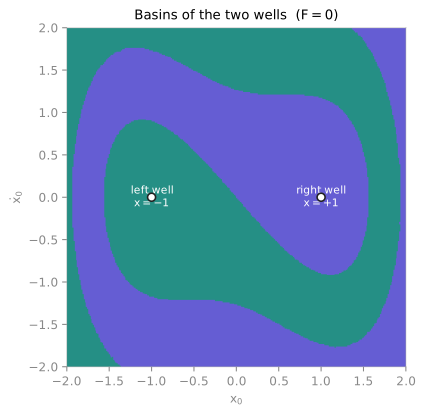
4. Paint the basins¶
ts.analysis.basins labels a lattice of initial
conditions by which attractor each one reaches — the basin map itself:
grid = data.Grid(np.array([-2.0, -2.0]), np.array([2.0, 2.0]), (300, 300))
basins = ts.analysis.basins(sys, grid, dt=0.5, max_steps=2000)

basins.n_attractors     # 2
basins.labels.shape     # (300, 300) — integer attractor id per initial condition
basins.fractions        # {1: 0.5001, 2: 0.4999}
labels is a plain integer array (id 1 and 2 here; -1 marks a diverged
cell), laid out on the grid you passed — ready to image directly:
# import matplotlib.pyplot as plt
# plt.imshow(basins.labels.T, origin="lower", extent=[-2, 2, -2, 2], cmap="coolwarm")
# plt.xlabel("$x_0$"); plt.ylabel(r"$\dot{x}_0$")
or, without touching matplotlib, through the result's own front door —
ts.plot(basins) returns a basins_image Plot
that renders itself with .plot() / .save("basins.png").
For a higher-dimensional flow you image a 2-D slice by passing a separate
full-dimension recurrence box and pinning the free axes of region with
counts == 1 — the recipe the magnetic-pendulum example on the
basins reference uses.
5. Quantify the boundary¶
How predictable is the outcome near the boundary? Three label-image diagnostics read the painted grid directly — no further integration:
ts.analysis.basin_fractions(sys, region, n_seeds=400, dt=0.5, max_steps=2000, seed=0)
# BasinFractions({1:0.53, 2:0.47}, diverged=0, n=400)      — basin stability

ts.analysis.basin_entropy(basins)
# BasinEntropy(Sb=0.04184, Sbb=0.4859, fractal_boundary=False)

ts.analysis.uncertainty_exponent(basins)
# UncertaintyExponent(alpha=0.9968, D0=1.003, R2=1.0)
Read them in turn:
basin_fractionsis Monte-Carlo basin stability (Menck et al., 2013): drawnrandom initial conditions and report each attractor's share. The two wells are near-symmetric, so the fractions sit close to \(\tfrac12, \tfrac12\) (this independent Monte-Carlo estimate, \(0.53 / 0.47\), differs from the full-gridbasins.fractionsabove only by sampling noise). Its standard error is \(\sqrt{p(1-p)/n}\) — dimension-free.basin_entropy(Daza et al., 2016) measures how mixed the labels are.fractal_boundary=Falsebecause the boundary entropy \(S_{bb} = 0.49\) stays below the \(\ln 2 \approx 0.69\) threshold: at this damping the boundary is a smooth curve.uncertainty_exponent(Grebogi et al., 1983) quantifies final-state sensitivity: perturbing an initial condition by \(\varepsilon\) flips its outcome with probability \(\sim \varepsilon^{\alpha}\). Here \(\alpha \approx 0.997\) is essentially \(1\), giving a boundary dimension \(D_0 = D - \alpha \approx 1.00\) — a genuine line (this fine \(300 \times 300\) grid resolves the smooth boundary cleanly; a coarser grid reads a slightly higher \(D_0\)).
A fourth, resilience, asks how far (in state space)
a given attractor is from its basin boundary — the smallest perturbation that
can knock the system out of it (Halekotte & Feudel, 2020):
When the boundary turns fractal
Smoothness is not guaranteed. Drive competing attractors hard enough — the
canonical case is a magnetic pendulum over three magnets, or Newton's method
on \(z^3 = 1\) — and the boundary becomes fractal and even Wada (every
boundary point touches all basins at once). Then basin_entropy reports
fractal_boundary=True (\(S_{bb} > \ln 2\)) and
wada_property detects the Wada structure. For our
two smooth basins ts.analysis.wada_property(basins) returns
WadaResult(is_wada=False, n_basins=2, W=0), as it should. The
Attractors & basins page walks the fractal case.
6. Tilt the potential — a tipping point¶
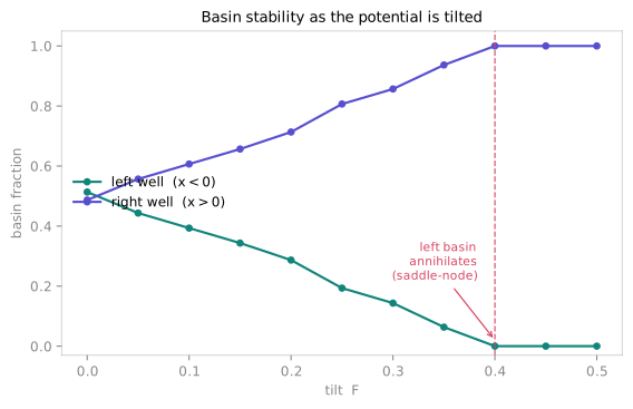
The basin picture is not fixed: change a parameter and it deforms, and a whole attractor — with its basin — can vanish. Our tilt \(F\) does exactly this. The cubic drift \(x - x^3 + F\) has three real roots (two wells plus the barrier) only while \(|F| < 2 / 3\sqrt{3} \approx 0.385\); past that, a saddle-node bifurcation destroys the shallower well.
continuation re-finds and matches the attractors at
each value of a swept parameter, tracking their basin fractions so a persisting
attractor keeps its id and a vanishing one drops to NaN (Datseris, Rossi &
Wagemakers, 2023):
cont = ts.analysis.continuation(sys, "F", np.linspace(0.0, 0.5, 11), region,
                       n_seeds=300, resolution=40, dt=0.5, max_steps=2000, seed=0)

cont.values            # array([0.  , 0.05, 0.1 , ..., 0.5 ])
cont.fractions[1]      # left well:  [0.51, 0.44, 0.39, ..., 0.06, nan, nan, nan]
cont.fractions[2]      # right well: [0.49, 0.56, 0.61, ..., 0.94, 1.0, 1.0, 1.0]
As the tilt grows the left well's basin steadily loses ground and then, between
\(F = 0.35\) and \(F = 0.40\), annihilates — its fraction falls to zero and its
id turns NaN. tipping_points reads that event off
the continuation:
ts.analysis.tipping_points(cont)
# CollectionResult(1 items)
#   {'value': 0.4, 'attractor': 1, 'kind': 'disappear',
#    'before': 0.06333..., 'after': 0.0}
One disappear event at \(F = 0.4\): the left well and its basin are gone, and
every initial condition now flows to the single surviving right well.
What you built¶
From three lines of math you produced the complete multistability portrait —
attractors, basins, basin stability, a quantified boundary, and a continuation
that catches the tipping point where a state disappears — every result
carrying its provenance in .meta. That is the path the whole toolkit is
designed around: define the system once, then compose
analysis on top.
Basins are for finite-dimensional states only
attractors / basins / continuation drive a map or
flow whose state is a point. A delay system (infinite-dimensional history)
or a stochastic system (no single deterministic limit) is rejected —
ts.analysis.attractors(ts.systems.OrnsteinUhlenbeck(), region) raises a
TypeError. For the stochastic analogue — noise hopping between the wells
of exactly this potential — see the
noise-driven tutorial.
See also¶
- Attractors & basins — the full basin / continuation / Wada API
- Fixed & periodic points — the equilibria these attractors are
- Noise-driven dynamics — the same double well, now with noise-induced switching
- The mental model — the definition contract in depth