Visualization · Animation

Animation¶

A trajectory moves. A static phase portrait is the whole orbit collapsed onto one page — every loop of the Lorenz butterfly drawn at once — which is exactly what you want for a figure but exactly wrong for building intuition, giving a talk, or watching a transient settle onto an attractor. TSDynamics turns any plot into a movie by attaching one small directive, and the semantic plot is otherwise untouched: the same PlotSpec that renders a still renders the animation, and a backend that cannot animate simply draws the final frame.

Animation is an orthogonal modifier. It is not a new PlotKind — a 3-D phase portrait stays a PHASE_PORTRAIT_3D, a time series stays a TIME_SERIES — it is an Animation object hung on spec.animation that says how the existing data plays over time. Because the directive is plain, serializable data it round-trips through to_dict/from_dict and ships to a web frontend untouched, and because it rides on the spec rather than a renderer, the same .trail(...) reads identically whether you export an mp4, an interactive HTML page, or a three.js viewer.

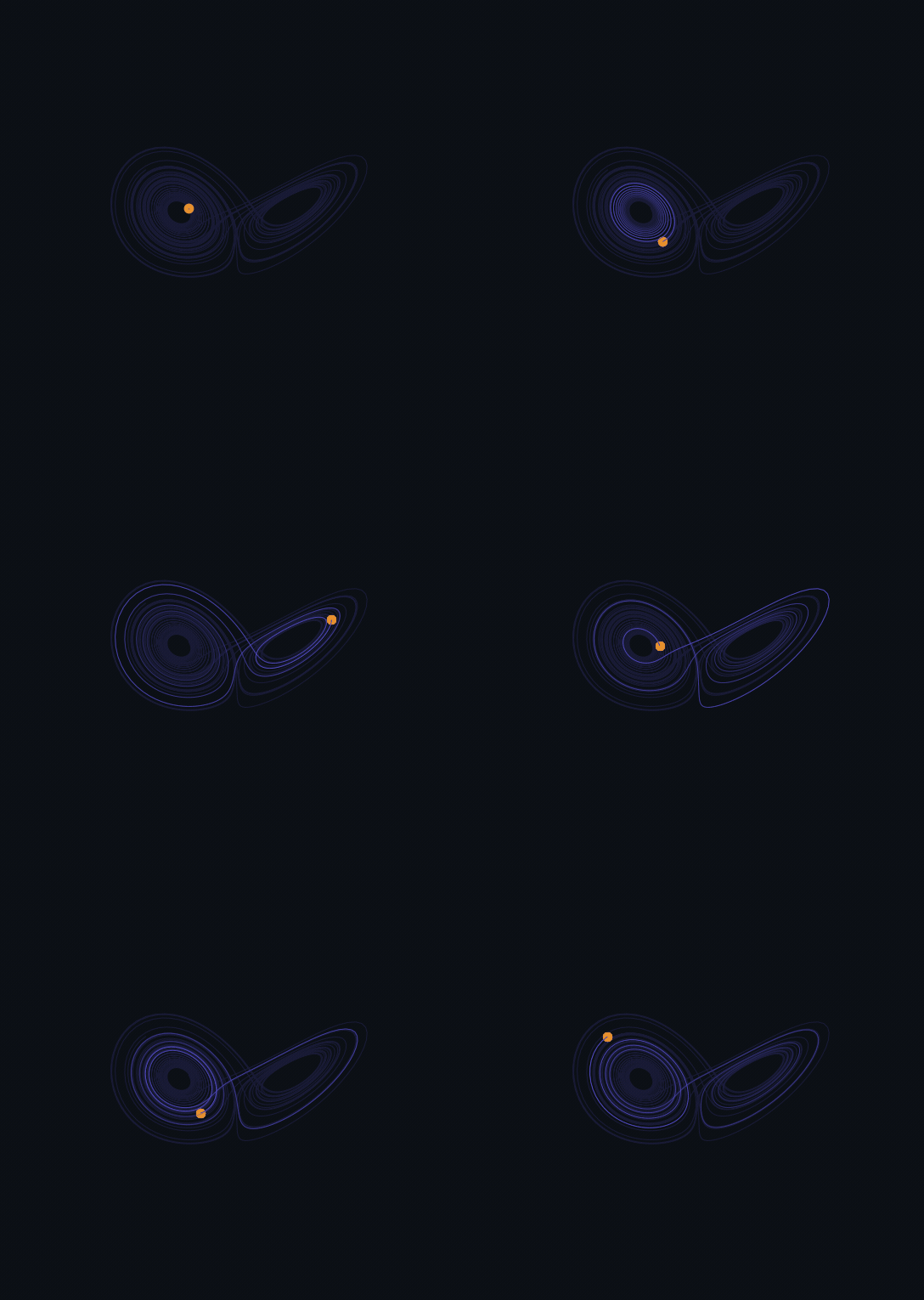
The Lorenz attractor drawing itself in as a looping reveal comet — an amber head tracing the orbit with a fading indigo tail on a dark stage, axes hidden — FIG 1 · a **reveal comet** of the Lorenz attractor: `to_plot_spec(animate=True)` keeps the full static curve and each frame shows a moving head (amber) with a fading tail reaching back 6 time units (indigo), axes hidden and drawn on the brand dark stage — the same "attractor floating in a dark room" look as the live WebGL viewer. Built by the exact snippet in the first example below and saved as a small looping GIF.

A first animation¶

The whole API hangs off one front-door argument. Every plot builder — Trajectory.to_plot_spec, system.to_plot_spec, ts.viz.plot — takes animate=, and animate=True stamps the default animation onto the spec:

import tsdynamics as ts

lor = ts.systems.Lorenz()
traj = lor.integrate(final_time=45.0, dt=0.01, ic=[1.0, 1.0, 1.0]).after(3.0)

spec = traj.to_plot_spec(components=["x", "y", "z"], animate=True)
spec.is_animated      # True — an Animation is attached
spec.kind             # PlotKind.PHASE_PORTRAIT_3D — the semantic kind is unchanged

The animate=True above is the figure at the top of the page, minus its styling. The committed version chains the fluent tweaks, hides the axes, and saves the GIF on the brand dark stage — every number below is the value the code actually produces:

AMBER, INDIGO, STAGE = "#E8912D", "#574FCF", "#0B0F14"

spec = (
    traj.to_plot_spec(components=["x", "y", "z"], animate=True)
    .animate(n_frames=100, fps=25)          # 100 frames at 25 fps -> a 4 s loop
    .trail(("time", 6.0), fade=True)        # tail reaches back 6 time units, fading
    .head(size=9.0, color=AMBER)            # amber "current state" marker
    .style(lw=0.8, axes=False)              # thin line, no axes
    .recolor(INDIGO)
    .camera(elev=22, azim=-60)              # a good butterfly angle
    .background(STAGE)                       # the dark stage (see the note below)
    .size(6.4, 6.0)
)
spec.save("lorenz-reveal.gif", dpi=85)      # .gif -> matplotlib FuncAnimation

Every method here mutates the spec and returns it, so the chain is one expression. They are the same fluent tweaks the styling page documents (.style, .recolor, .size, .background) plus the animation-specific ones (.animate, .trail, .head, .camera) covered here.

Animate on a solid background, not a transparent one

A GIF has no real alpha channel — a transparent figure is flattened to a single fill colour by the encoder, which many viewers render as a jarring green. Give an animation an explicit solid background so it lands on a clean stage: .background("#0B0F14") (the brand dark) here, or any colour / a .theme(...). The committed hero loops all use the dark stage, matching the WebGL viewers. A still .png/.svg save is unaffected (it keeps real transparency).

A gallery¶

The same one-directive API drives every kind of motion. Each loop below is built by the exact snippet beside it — an IC- or seed-pinned trajectory, a fluent .animate/.trail/.head/.camera chain, and a .background("#0B0F14") stage — and lives in docs/_tooling/make_viz_figures.py.

A spinning attractor that accretes¶

camera(spin=…) sweeps the azimuth over the loop while a persistent trail (.trail(None)) draws the whole orbit in and keeps it — the elegant "watch it accrete while it turns" hero shot. Camera spin is a matplotlib-only knob.

The Aizawa attractor accreting as a teal orbit on a dark stage while the camera makes one full revolution, an indigo state head leading the reveal — FIG 2 · the **Aizawa** attractor with `.trail(None)` (persistent — nothing erases) and `.camera(spin=1.0)`: one full revolution over the loop as the teal orbit draws itself in, an indigo head leading.

import tsdynamics as ts

TEAL, INDIGO = "#2CC5AE", "#574FCF"
aiz = ts.systems.Aizawa()
traj = aiz.integrate(final_time=95.0, dt=0.01, ic=[0.1, 0.0, 0.0]).after(15.0)

spec = (
    traj.to_plot_spec(components=[0, 1, 2], animate=True)   # Aizawa has no named vars
    .animate(n_frames=100, fps=25)
    .trail(None)                          # persistent — the orbit accretes and stays
    .head(size=9.0, color=INDIGO)
    .camera(elev=18, azim=-70, spin=1.0)  # one full revolution over the loop
    .style(lw=0.7, axes=False)
    .recolor(TEAL)
    .background("#0B0F14")
    .size(6.0, 6.0)
)
spec.save("aizawa-spin.gif", dpi=74)

A pattern-formation field movie¶

The "frames" model (below) plays a spatially-extended system's field over time. Gray–Scott's activator grows and divides into a Turing pattern — genuinely striking, and honest: each frame is a real spatial snapshot, not a comet.

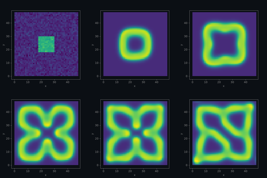
A Gray-Scott reaction-diffusion field evolving over time: viridis spots on a dark-blue field grow, replicate, and organise into a maze-like Turing pattern — FIG 3 · a **Gray–Scott** reaction–diffusion field played frame by frame with `kind="field", animate=True` — the activator self-replicates into a Turing pattern (viridis). This is the `frames` model, covered below.

import tsdynamics as ts

# GrayScott has a deterministic seeded IC, so the pattern is reproducible.
gs = ts.systems.GrayScott()
gtr = gs.integrate(final_time=4000.0, dt=85.0)     # a 48x48 reaction-diffusion field

spec = (
    gtr.to_plot_spec(kind="field", animate=True)   # SPATIAL_FIELD, mode="frames"
    .animate(fps=14)
    .style(cmap="viridis")
    .background("#0B0F14")
    .size(4.6, 4.6)
)
spec.save("gray-scott-field.gif", dpi=78)

A delay-embedding reveal¶

A scalar delay system's true state lives in an infinite-dimensional history space; the delay embedding x(t) vs x(t − τ) reconstructs its attractor, and a comet sweeps it in.

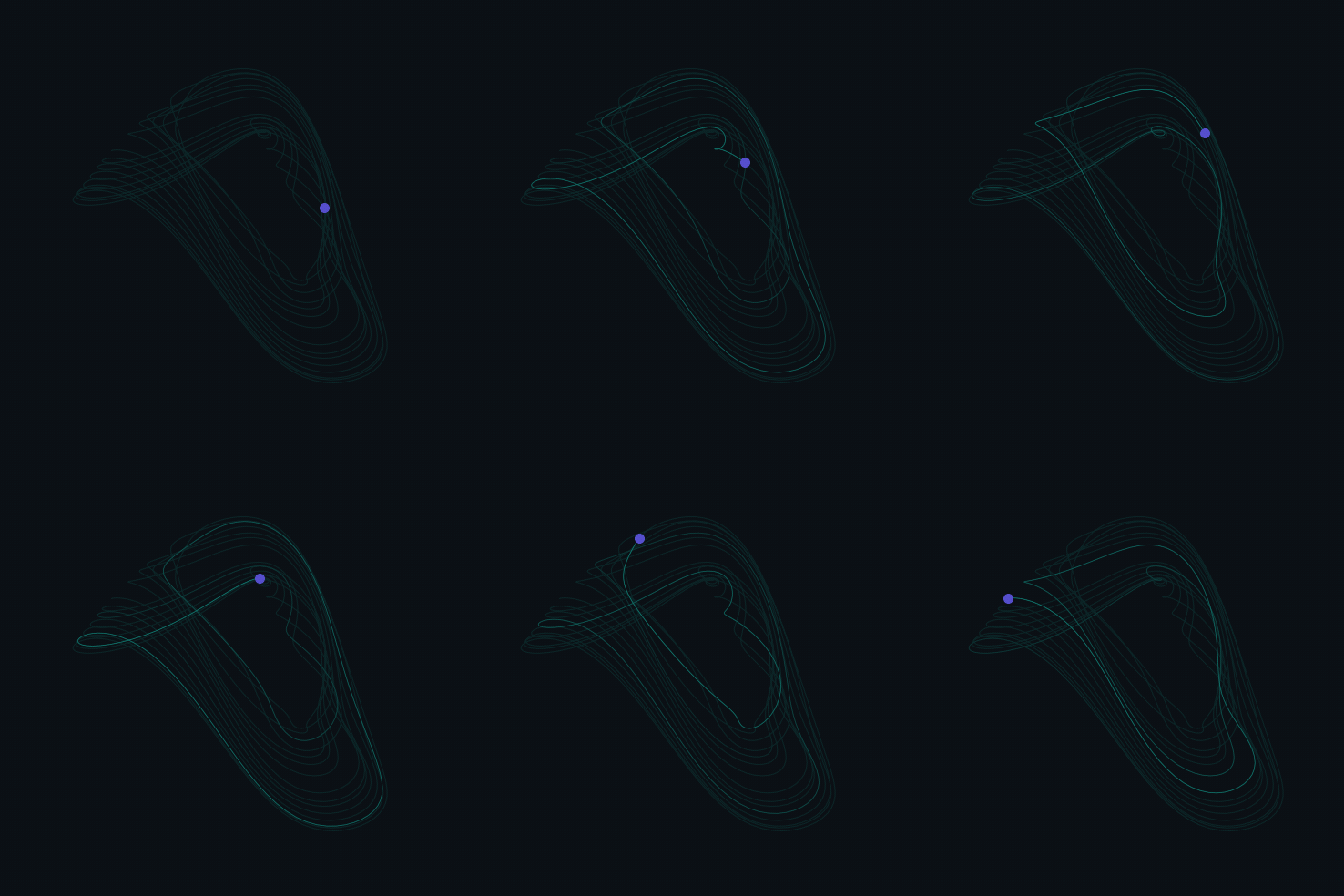
A Mackey-Glass delay embedding drawing itself in: a teal comet with an indigo head traces the folded chaotic band on a dark stage — FIG 4 · the **Mackey–Glass** delay embedding `x(t)` vs `x(t − 17)`, revealed as a teal comet with an indigo head — the folded chaotic band of a DDE reconstructed from one scalar signal.

import numpy as np
import tsdynamics as ts

mg = ts.systems.MackeyGlass()
traj = mg.integrate(
    final_time=900.0, dt=0.5,
    history=lambda s: [1.0 + 0.1 * np.sin(0.2 * s)],
).after(150.0)

spec = (
    traj.to_plot_spec(kind="delay", components="x", tau=17.0, animate=True)
    .animate(n_frames=100, fps=25)
    .trail(("time", 120.0), fade=True)
    .head(size=8.0, color="#574FCF")
    .style(lw=0.6, axes=False)
    .recolor("#2CC5AE")
    .background("#0B0F14")
    .size(5.6, 5.6)
)
spec.save("mackey-glass-delay.gif", dpi=88)

A two-panel lockstep composite¶

A composite plays every panel on one master clock. Here the state head on the 3-D butterfly and the sweep on its own x(t) trace advance together — the same instant shown two ways. Passing a fully-built Animation at compose time propagates the whole timeline (frame count and trail) into each panel, with the per-kind head default (a head on the portrait, none on the time series).

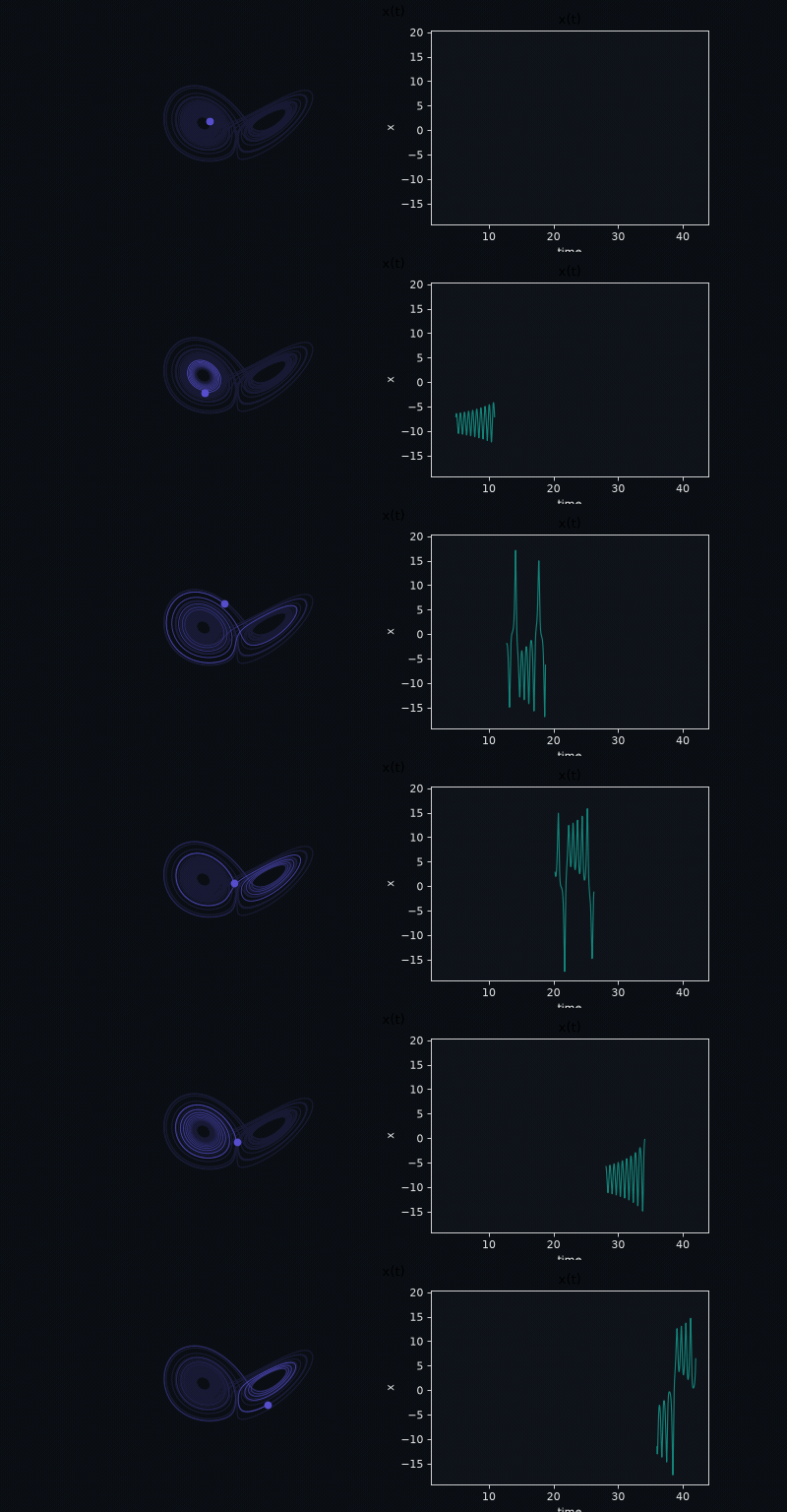
A two-panel movie: left, the Lorenz butterfly revealing as an indigo comet; right, its x(t) time series sweeping in teal, both advancing on one shared clock — FIG 5 · a **lockstep composite** via `ts.viz.plot(portrait, trace, layout="row", animate=Animation(...))`: the 3-D Lorenz reveal (indigo) and its `x(t)` trace (teal) play on one master clock — the head on the butterfly and the sweep on the trace are the same instant.

import tsdynamics as ts
from tsdynamics.viz import get_theme, plot
from tsdynamics.viz.producers import time_series
from tsdynamics.viz.spec import Animation

lor = ts.systems.Lorenz()
traj = lor.integrate(final_time=42.0, dt=0.01, ic=[1.0, 1.0, 1.0]).after(3.0)

portrait = (
    traj.to_plot_spec(components=["x", "y", "z"])
    .style(lw=0.7, axes=False).recolor("#574FCF").camera(elev=22, azim=-60)
)
portrait.relabel(title="")
trace = time_series(traj, components=["x"]).style(lw=1.0).recolor("#2CC5AE")
trace.relabel(title="x(t)", x="time", y="x")
# keep the visible time-series axes legible on the dark stage
trace.theme(get_theme("dark"))

# A fully-built master Animation so both panels inherit frame count AND trail.
master = Animation(n_frames=100, fps=25, trail_kind="time", trail_length=6.0, trail_fade=True)
comp = plot(portrait, trace, layout="row", animate=master).size(8.0, 4.1)
comp.save("lorenz-composite.gif", dpi=80)

`animate=` — three ways to attach¶

animate= accepts three forms, in increasing order of control:

Form	Meaning
`animate=True`	Attach the per-kind defaults (see below).
`animate={...}`	A dict overriding individual `Animation` fields on top of the defaults.
`animate=Animation(...)`	A fully built `Animation`, used verbatim.

from tsdynamics.viz.spec import Animation

# defaults
a = traj.to_plot_spec(components=["x", "y", "z"], animate=True)

# a dict tweaks specific fields (the rest stay at their per-kind defaults)
b = traj.to_plot_spec(components=["x", "y", "z"], animate={"fps": 24, "n_frames": 60})
b.animation.fps          # 24
b.animation.n_frames     # 60

# an Animation is copied in verbatim
c = traj.to_plot_spec(components=["x", "z"], animate=Animation(fps=15, spin=1.0))
c.animation.spin         # 1.0

The Animation passed in is copied, never stored by reference, so a later .trail(...)/.head(...) on the spec does not reach back and mutate your object.

Either build the animation at the front door with animate=, or attach it afterwards with the fluent .animate() — calling .animate() on a static spec makes it animated with the same defaults. The two are equivalent:

# these produce the same spec
traj.to_plot_spec(components=["x", "y", "z"], animate=True)
traj.to_plot_spec(components=["x", "y", "z"]).animate()

Per-kind defaults¶

animate=True picks sensible defaults by plot kind so the common case needs no tuning:

A windowed comet — a moving head plus a short trailing tail over the full faint curve. The tail defaults to ("steps", …) ≈ 1/10 of the series length, capped at 200 samples, which keeps the comet crisp and (for the interactive backends) the export small.
The head marker is on for everything except a plain time series — a moving dot makes sense on a phase portrait or a spacetime sweep line, but a time series reads better as a bare growing curve.
A spatial-field spec always animates in the frames model (the field movie) regardless of the other defaults.

d = traj.to_plot_spec(components=["x", "y", "z"], animate=True)
d.animation.trail_kind      # 'steps'
d.animation.trail_length    # 200.0   (min(n_steps // 10, 200); n_steps = 4201)
d.animation.head            # True    (a 3-D portrait)

e = traj.to_plot_spec(components="x", animate=True)   # a TIME_SERIES
e.animation.head            # False   (a bare growing curve)

A persistent "orbit draws itself in" — the classic reveal where nothing ever erases — is one tweak away: .trail(None), covered next.

The reveal model — comets, trails, heads¶

The default frame model is "reveal". The layer keeps its full static data and each frame shows a slice of it: the head sits at the current sample, and a tail reaches back behind it. O(data) memory — nothing is recomputed per frame. It covers every trajectory-shaped plot: phase portraits, delay embeddings, time series, and spacetime images (where the "head" is a sweep line).

Three fluent methods shape the comet.

`.animate(...)` — the timeline¶

spec.animate(
    fps=30,              # playback frames per second
    n_frames=120,        # explicit frame count (wins over duration)
    duration=None,       # OR total seconds — with fps this fixes the frame count
    loop=True,           # repeat forever
    pingpong=False,      # play forward then reverse each loop
    mode="reveal",       # "reveal" (comet) or "frames" (field movie)
)

The frame count resolves as: n_frames if given, else round(duration * fps), else a capped default — always clamped to at most the number of samples (you cannot reveal more distinct points than exist):

s = traj.to_plot_spec(components="x", animate=True).animate(duration=4.0, fps=30)
s.animation.frame_count(len(traj.t))   # 120  (= 4.0 * 30)

pingpong=True mirrors the frame sequence — forward, then back — for a seamless there-and-back loop:

a = Animation(n_frames=5, pingpong=True)
a.head_indices(100)     # [0, 25, 50, 74, 99, 74, 50, 25]  (forward then reverse)

`.trail(length, *, fade)` — the tail behind the head¶

The tail length is given in physical time units or sample steps, or None for a persistent trail that never erases:

spec.trail(("time", 6.0))     # tail reaches back 6.0 time units
spec.trail(("steps", 300))    # tail is the last 300 samples
spec.trail(None)              # persistent — the curve draws itself in and stays
spec.trail(("time", 6.0), fade=True)   # + fade the tail opacity from head to tail

A "time" length is converted to a sample count using the trajectory's dt (recorded on meta["dt"], so it resolves at render time). A persistent trail resolves to None samples — the whole revealed curve is kept:

persistent = traj.to_plot_spec(components=["x", "y", "z"], animate=True).trail(None)
persistent.animation.tail_samples(0.01)   # None  (keep everything revealed so far)

windowed = traj.to_plot_spec(components=["x", "y", "z"], animate=True).trail(("time", 6.0))
windowed.animation.tail_samples(0.01)     # 600   (6.0 / 0.01)

`.head(...)` — the moving "current state" marker¶

spec.head(show=True, size=7.0, color="#E8912D", symbol="o")

color=None (the default) inherits the layer colour; pass an explicit colour — as the top figure does with amber against an indigo trail — to make the head pop. show=False drops the marker for a pure trailing curve.

The tail window is a speed and size lever

A short tail (("steps", 200)) keeps the comet crisp and, for the plotly and three.js exports, keeps the streamed data tiny — the interactive page only ever holds a sliding window. A persistent trail (.trail(None)) is the most dramatic ("watch the whole attractor accrete") but the heaviest. Reach for a windowed comet for a talk loop and a persistent trail for a single hero shot.

3-D camera — angle and spin¶

For a 3-D spec, .camera(...) sets a fixed viewing angle and/or an animated spin:

spec.camera(elev=22, azim=-60)   # a fixed angle (static — recorded in meta["camera"])
spec.camera(spin=2.0)            # revolve the camera 2 full turns over the animation

elev/azim are a static tweak (they apply to a still too); spin is the animated one — it makes the azimuth sweep spin full turns over the whole playback, and setting it turns animation on:

orbit = traj.to_plot_spec(components=["x", "y", "z"]).camera(elev=22, azim=-60, spin=2.0)
orbit.is_animated          # True — spin implied an animation
orbit.animation.spin       # 2.0
orbit.meta["camera"]       # {'elev': 22.0, 'azim': -60.0}

Camera spin is a matplotlib feature. In the interactive backends you orbit the camera yourself while the comet plays (see export targets), so a scripted spin is unnecessary there.

A live time readout — `.clock(...)`¶

.clock() draws a time label that updates each frame — useful when the physical time, not just the frame index, carries meaning (a forced oscillator, a slow transient):

spec.clock(fmt="t = {t:.1f}s")    # {t} is the current time
spec.animation.clock              # True
spec.animation.clock_format       # 't = {t:.1f}s'

The {t} field is the current physical time, read from the trajectory grid. The clock is a matplotlib-only overlay (like camera spin).

Hiding the axes — `.style(axes=False)`¶

Not animation-specific, but the reason most attractor movies read well: .style(axes=False) hides the ticks, labels, gridlines, and (in 3-D) the grey background panes, for a clean "object floating in space" look. Every renderer honors it — matplotlib turns the axes off, plotly sets the scene axes invisible, three.js drops its grid. The top figure uses it; so should most hero loops.

spec = (
    traj.to_plot_spec(components=["x", "y", "z"], animate=True)
    .style(lw=0.6, axes=False)      # thin line, no axes
    .recolor("#574FCF")
)

The spatial-field movie¶

A spatially-extended system — a method-of-lines PDE whose state vector is a flattened field — animates differently. There is no comet: each frame is the field's spatial state at that instant, so consecutive frames carry genuinely different data. This is the "frames" frame model, and it is reached through the kind="field" recipe:

gs = ts.systems.GrayScott()
gtr = gs.integrate(final_time=1500.0, dt=5.0)      # a 48x48 reaction-diffusion field

movie = gtr.to_plot_spec(kind="field", animate=True)
movie.kind                 # PlotKind.SPATIAL_FIELD
movie.animation.mode       # 'frames'  (forced — the field IS the motion)
movie.animation.head       # False     (no comet, no head marker)
movie.layers[0].data["frames"].shape   # (T, 48, 48) — every per-time snapshot stacked

FIG 3 above is exactly this — the Gray–Scott activator field played frame by frame. The per-frame plot follows the field's spatial dimensionality, dispatched from the system's _field_shape metadata (recorded on meta["field_shape"] at integration time):

A 2-D field u(x, y) — Gray–Scott, Swift–Hohenberg — plays as an imshow heatmap movie.
A 1-D field u(x) — Kuramoto–Sivashinsky — plays as a travelling-wave line (the moving spatial profile).

import numpy as np

ks = ts.systems.KuramotoSivashinsky()
ic = 0.1 * np.cos(np.linspace(0.0, 2.0 * np.pi, ks.dim, endpoint=False))
ktr = ks.integrate(final_time=150.0, dt=0.5, ic=ic).after(20.0)

wave = ktr.to_plot_spec(kind="field", animate=True)
wave.kind                             # PlotKind.SPATIAL_FIELD
wave.layers[0].data["frames"].shape   # (T, 32) — a 1-D profile stacked over time
wave.save("ks-wave.gif")

The static save of a field movie is the final field — a .png of a kind="field" spec is the last snapshot — so a still and a movie share one spec. A multi-block field state (Gray–Scott packs an activator v and inhibitor u) declares field_labels; components="u" / "v" picks the block, defaulting to the last (the activator). See the Visualization overview for the static two-panel spatial-field showcase (a Gray–Scott heatmap beside a Kuramoto–Sivashinsky space–time diagram).

The field movie is matplotlib-only

The frames model plays through the matplotlib renderer (mp4 / gif). Plotly declines an animated SPATIAL_FIELD and draws the static final field instead; three.js draws a 1-D profile and declines a 2-D field. For a shared, interactive field explorer, export the static heatmap and animate offline.

Export targets¶

spec.save(path) picks the backend from the file extension. The routing differs for an animated spec:

Extension	Backend	What you get
`.mp4` / `.gif`	matplotlib	A rendered video / looping GIF (`FuncAnimation`, written via ffmpeg / pillow).
`.html`	plotly	A self-contained, real-time interactive page — the comet streams and you can orbit the 3-D camera while it plays.
three.js (`.json`)	three.js exporter	A geometry payload plus a `metadata.animation` block a WebGL loader plays as a reveal comet.
`.png` / `.svg` / `.pdf`	matplotlib	The final frame (the fully-revealed curve / final field) — an animated spec still makes a clean still.

spec.save("orbit.gif")     # looping GIF (matplotlib)
spec.save("orbit.mp4")     # video (matplotlib, needs ffmpeg)
spec.save("orbit.html")    # interactive real-time comet (plotly)
spec.save("orbit.png")     # the final, fully-revealed frame (matplotlib)

fps, dpi, and size can be overridden on the save call for that write only:

spec.save("orbit.mp4", fps=60, dpi=150, size=(1280, 720))

matplotlib — mp4 / gif¶

The reference animator builds a FuncAnimation and writes it with the writer inferred from the extension (ffmpeg for .mp4, pillow for .gif). This is the path that honors camera spin, the clock, and the spatial-field movie — the features the interactive backends do not carry. The GIF at the top of this page is exactly this path at dpi=80.

plotly — real-time interactive HTML¶

spec.save("x.html") on an animated spec writes a self-contained page whose comet is streamed in real time by mutating the trace buffers in place. The full attractor is drawn once (static, and for 3-D fully rotatable), and a requestAnimationFrame loop advances a windowed comet plus a single-point head over it. A minimal play/pause + restart overlay with a percent readout makes it obviously alive.

The honest fact about 3-D here: plotly's WebGL 3-D traces cannot be streamed while you orbit — every per-frame 3-D update forces a full scene replot that would eat the drag gesture. So the loop pauses the comet stream for the duration of a drag and resumes on release from where it paused, leaving the scene free to orbit as smoothly as a static plot. You get both — a playing comet and a rotatable camera — just not simultaneously mid-drag. 2-D plots have no orbit gesture and stream continuously.

three.js — a `metadata.animation` block¶

The three.js exporter adds an animation block to metadata when the spec is animated; the geometry buffers are byte-identical to the static export. The reference WebGL loader plays it as a reveal comet — a faint full-curve backdrop, a bright windowed trail advanced by setDrawRange, and a moving head point — on its own animation clock, and because the draw-range update is independent of the orbit controls, the camera is held still by default yet orbitable while it plays:

from tsdynamics.viz.render import render_spec

spec = traj.to_plot_spec(components=["x", "y", "z"], animate=True).animate(fps=30).trail(("time", 4.0))
payload = render_spec(spec, "threejs")
"animation" in payload.payload["metadata"]      # True
sorted(payload.payload["metadata"]["animation"])
# ['duration', 'fps', 'head', 'head_color', 'head_size', 'loop',
#  'n_frames', 'n_samples', 'pingpong', 'trail_length_samples']

The reveal sweeps a line index buffer, so the block is emitted only for LINE / LINE3D specs. An animated points-only or surface-only spec has no comet to sweep, so the exporter drops to a static payload and warns (VisualizationDegraded) rather than silently pretending to animate:

import warnings
from tsdynamics.viz.producers import spacetime

img = spacetime(traj).animate(fps=10)     # a SPACETIME (IMAGE) — no line to sweep
with warnings.catch_warnings(record=True) as w:
    warnings.simplefilter("always")
    payload = render_spec(img, "threejs")
"animation" in payload.payload["metadata"]   # False — a static export
# w carries one VisualizationDegraded warning

Serialization¶

Because the Animation is plain data, an animated spec round-trips losslessly. The directive survives to_dict/from_dict, so a computed animation can be cached, shipped to a web frontend, or replotted without recomputation — and it adds no new PlotKind (the frozen plot-kind vocabulary is untouched):

from tsdynamics.viz.spec import PlotSpec

spec = (
    traj.to_plot_spec(components=["x", "y", "z"], animate=True)
    .animate(fps=25, n_frames=50)
    .trail(("steps", 300))
)
d = spec.to_dict()
d["animation"]["fps"]        # 25.0

rt = PlotSpec.from_dict(d)
rt.is_animated               # True
rt.animation.trail_kind      # 'steps'

Reference — the `Animation` fields¶

Every fluent tweak above sets one or more fields on the Animation directive. The full set, with defaults:

Field	Default	Set by	Meaning
`fps`	`30.0`	`.animate(fps=)`	Playback frames per second.
`duration`	`None`	`.animate(duration=)`	Total seconds; with `fps` fixes the frame count.
`n_frames`	`None`	`.animate(n_frames=)`	Explicit frame count (wins over `duration`/`fps`).
`loop`	`True`	`.animate(loop=)`	Repeat forever.
`pingpong`	`False`	`.animate(pingpong=)`	Play forward then reverse each loop.
`mode`	`"reveal"`	`.animate(mode=)`	Frame model — `"reveal"` (comet) or `"frames"` (field movie).
`trail_kind`	`None`	`.trail(length=)`	Tail units — `"time"`, `"steps"`, or `None` (persistent).
`trail_length`	`None`	`.trail(length=)`	Tail length in the chosen units.
`trail_fade`	`False`	`.trail(fade=)`	Fade the tail opacity from head to tail.
`head`	`True`	`.head(show=)`	Draw the moving "current state" marker.
`head_size`	`6.0`	`.head(size=)`	Head marker size.
`head_color`	`None`	`.head(color=)`	Head colour (`None` inherits the layer colour).
`head_symbol`	`"o"`	`.head(symbol=)`	Head marker symbol.
`spin`	`0.0`	`.camera(spin=)`	Camera revolutions over the animation (3-D, matplotlib).
`clock`	`False`	`.clock(show=)`	Draw a live time readout (matplotlib).
`clock_format`	`"t = {t:.2f}"`	`.clock(fmt=)`	Clock label format (`{t}` = current time).

Pitfalls¶

animate=True on a spatial-field spec is a field movie, not a comet. The "frames" model is forced for a SPATIAL_FIELD — you cannot put a comet on a PDE field, and asking for one is silently coerced to the field movie.
Camera spin and the clock are matplotlib-only. Export those to .mp4 / .gif. In plotly you orbit the camera by hand; a scripted spin is ignored.
.mp4 needs ffmpeg on the PATH; .gif uses pillow (a hard dependency, always available). Reach for .gif when ffmpeg is not installed.
A three.js animation only plays for a line. A points- or surface-only animated spec exports as a static payload with a VisualizationDegraded warning — it does not silently drop the frames.
Always pin an explicit ic= (or a seed= for a stochastic system) when a movie's shape must be reproducible — many catalogue systems draw a random IC each run, so an un-pinned attractor movie is a different orbit every time.