Tutorial · Reconstruction from one signal

Reconstruction from one signal¶

The first two tutorials had the luxury every textbook has and no experiment ever does: the equations. Real data arrives the other way round. You have a single recorded channel — a voltage, a concentration, a light curve — sampled over time, and nothing else. No state vector, no model, no idea whether the wiggle in front of you is a deterministic system worth analysing or just filtered noise.

This tutorial walks the whole inference the other direction: from one scalar \(x(t)\) back to the geometry and invariants of the system that produced it. We will reconstruct the attractor from the single channel, choose the two reconstruction parameters with principled heuristics, measure the attractor's fractal dimension and its largest Lyapunov exponent from the recording, and finish with the question that should always come first — is this even nonlinear, or could coloured noise fake it?

To keep it honest and reproducible we generate the mystery signal from a known system (the Rössler flow) and then immediately throw the model away, keeping only one component. Everything after that line uses the scalar alone — so we can check every recovered number against the truth at the end.

import numpy as np
import tsdynamics as ts

# generate a trajectory, then keep ONLY the x channel — pretend this is all you recorded
full = ts.systems.Rossler().integrate(final_time=400.0, dt=0.05, ic=[1.0, 0.0, 0.0])
x = full.y[1000:, 0]        # a single scalar signal, transient dropped
x.shape                     # (7001,)

From here on, x is the only thing we touch.

1. The theorem that makes it possible¶

You would think one channel throws away most of the state. Takens' embedding theorem (Takens, 1981) says otherwise: from one generic observable of a deterministic system you can reconstruct a trajectory whose attractor is diffeomorphic to the true one — same topology, same invariants — simply by stacking time-delayed copies of the single signal into a vector,

\[ \mathbf{y}_i = \big(x_i,\; x_{i+\tau},\; x_{i+2\tau},\; \dots,\; x_{i+(m-1)\tau}\big). \]

Two choices make the reconstruction faithful: the delay \(\tau\) and the embedding dimension \(m\). The delay-embedding tools give a principled way to pick each.

2. Choose the delay¶

The delay trades two failures against each other. Too small, and \(x_i\) and \(x_{i+\tau}\) are nearly identical — the reconstruction collapses onto the diagonal. Too large, and on a chaotic signal they become causally unrelated — the geometry folds noise into itself. The recommended criterion is the first local minimum of the time-delayed mutual information (Fraser & Swinney, 1986): the lag at which the next coordinate adds the most new information while staying dynamically related to the current one.

tau = ts.optimal_delay(x, method="mi", max_delay=120)   # 27 samples

mi = ts.mutual_information(x, max_delay=120)
mi.optimal_lag          # 27   — the same lag, read off the I(tau) curve
# mi.plot()             # inspect the curve, with the chosen tau marked

optimal_delay returns a CountResult that is the integer \(\tau = 27\), so it drops straight into embed. The linear alternative — the autocorrelation \(1/e\) rule, method="acf" — gives \(\tau \approx 22\) here, close to the mutual-information choice; when they disagree, prefer the mutual-information lag, which sees nonlinear dependence the autocorrelation misses.

3. Choose the dimension¶

The dimension must be large enough to unfold the attractor — to remove the false crossings a too-flat projection creates where two distant states happen to overlap. Cao's method (Cao, 1997) and Kennel's false nearest neighbours (Kennel et al., 1992) both detect the smallest \(m\) at which those artefacts vanish, unified behind embedding_dimension:

m_fnn = ts.embedding_dimension(x, method="fnn", delay=tau, max_dim=8)
int(m_fnn)              # 3   — Kennel FNN; matches Rössler's true dimension

m_cao = ts.embedding_dimension(x, method="cao", delay=tau, max_dim=8)
int(m_cao)             # 4   — Cao's conservative saturation threshold
# m_cao.plot()         # the E1/E2 saturation curves, with the chosen m marked

The two estimators need not agree to the integer — Cao's saturation threshold and Kennel's tolerance are conservative in different directions — so on a marginal case read \(m\) off the shape of the diagnostic curve rather than trusting a single number, and when in doubt embed one dimension higher. Here FNN recovers the true dimension 3 exactly; we take \(m = 3\).

4. Reconstruct — one channel becomes an attractor¶

With both parameters chosen, embed builds the matrix of delay vectors:

emb = ts.embed(x, dimension=3, delay=tau)
emb.shape               # (6947, 3) — one reconstructed state per row, in time order

The returned Embedding behaves as that bare array, so it drops straight into any point-set analysis. The two leading columns \((x_i,\,x_{i+\tau})\) are the reconstructed plane — plot them and the folded Rössler loop reappears, rebuilt from the single channel. Because a Trajectory can build the same delay view directly, you can eyeball the reconstruction with the plotting front door:

# the x(t) vs x(t - tau) delay portrait, straight from the trajectory
full.to_plot_spec(kind="delay", components="x", tau=tau * 0.05).save("delay.png")

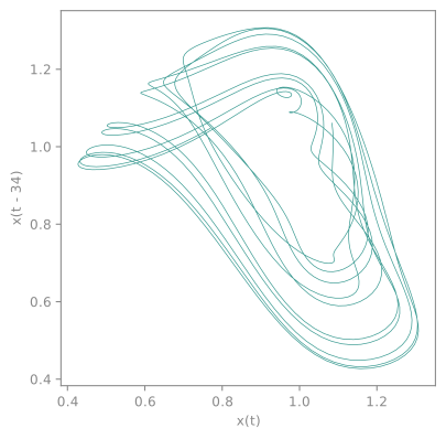
A delay-coordinate reconstruction of a flow from one channel — FIG 1 · a delay embedding — x(t) against x(t − τ) — built from a single recorded channel. The `kind="delay"` recipe takes τ in *time units* (here τ = 27 samples × dt = 1.35). The loop is the reconstructed attractor: same topology as the true state space, from one signal.

5. Measure the attractor — from the reconstruction¶

Now the payoff. Takens guarantees the reconstruction preserves the invariants, so any quantity that depends only on the attractor's geometry or dynamics can be computed from the embedded cloud — no equations needed.

Fractal dimension. The correlation dimension (Grassberger & Procaccia, 1983) reads off the point cloud directly. On a reconstructed flow you must set a Theiler window, because temporally adjacent samples sit spuriously close and bias the estimate downward — a few delays is a safe choice:

ts.correlation_dimension(emb, theiler=tau)     # ≈ 1.74   (Rössler D2, from x alone)

Largest Lyapunov exponent. lyapunov_from_data estimates the top exponent from how fast embedded neighbours diverge (Kantz, 1994). Pass the sampling interval dt= so the rate comes out per unit time, and — crucially — inspect the stretching curve before quoting a number:

res = ts.lyapunov_from_data(x, dimension=3, delay=tau, dt=0.05, k_max=80)
res.times, res.divergence      # the S(k) curve — plot it, find the linear stretch

The curve \(S(k)\) rises, flattens, then climbs into a clean linear region roughly between look-ahead times \(0.3\) and \(1.3\) (sample indices 6–26). The exponent is the slope of that stretch, not of the whole curve — fit it explicitly:

res = ts.lyapunov_from_data(x, dimension=3, delay=tau, dt=0.05, k_max=80, fit=(6, 26))
float(res)             # ≈ 0.074   per unit time — positive, so chaotic

Never quote the automatic fit blind

On a flow the divergence curve typically overshoots before it settles, so the default automatic fit overestimates (here it returns \(\approx 0.13\), well above the truth). The estimate is only as good as the scaling region you choose — always look at res.times vs res.divergence and pass an explicit fit=(lo, hi) before quoting a publishable value. This is the place from-data exponents go wrong.

How did we do? We can cheat now and check against the model we threw away:

# the truth, from the full state and the equations
ts.correlation_dimension(full.y[1000:], theiler=tau)                     # ≈ 1.75
float(ts.max_lyapunov(ts.systems.Rossler(ic=[1.0, 0.0, 0.0]), dt=0.05, seed=0))  # ≈ 0.062

\(D_2 = 1.74\) from one channel versus \(1.75\) from the full state; \(\lambda \approx 0.074\) from the recording versus the true \(\approx 0.06\)–\(0.07\) (literature: \(0.071\)). One scalar signal, and we recovered both invariants to within their estimation error.

6. The prior question: is it even nonlinear?¶

Everything above assumes the signal came from a deterministic nonlinear system. But a correlation dimension and a Lyapunov exponent will happily return finite numbers for coloured noise too — a linear stochastic process with a spectral peak can mimic a low-dimensional oscillation. Before trusting any of it, you should test the null hypothesis that the data is linear.

The surrogate-data method (Theiler et al., 1992) does exactly this: generate an ensemble of surrogates that reproduce the data's linear fingerprint (its amplitude distribution and power spectrum) but are otherwise random, compute a nonlinearity-sensitive statistic on the data and on each surrogate, and reject the linear null if the data sits in the tail.

res = ts.surrogate_test(x, statistic="prediction_error",
                        method="iaaft", n=39, seed=0)

res.p_value      # ≈ 0.025   — data lands in the tail of the null
res.z_score      # ≈ -36     — vastly more predictable than any surrogate
res.rejected     # True      → linear-stochastic null rejected

The prediction_error statistic measures how well a locally-constant predictor forecasts the series in its embedding. Deterministic data is more predictable than its phase-randomised surrogates, so the data sits far below the null — the linear hypothesis is rejected. The nonlinear analysis was justified.

The control matters just as much: a genuinely linear process must pass. A resonant AR(2) process is coloured noise with a spectral peak — exactly the thing that could fake an attractor — and the test correctly clears it:

rng = np.random.default_rng(0)
noise = np.zeros(7000)
for i in range(2, 7000):                       # AR(2), a resonant linear process
    noise[i] = 1.6 * noise[i-1] - 0.95 * noise[i-2] + rng.standard_normal()

ts.surrogate_test(noise, statistic="prediction_error",
                  n=39, seed=1).rejected        # False — linear null NOT rejected

Coloured noise passes; the Rössler signal does not. That contrast is the whole point: a surrogate test that "rejects everything" is broken, not sensitive. Run the test first on real data — it tells you whether the rest of the pipeline is measuring dynamics or fitting noise.

What you built¶

Starting from a single scalar channel with the model discarded, you rebuilt the attractor by delay embedding, chose \(\tau\) and \(m\) from mutual information and false-nearest-neighbours, measured the correlation dimension (\(1.74\)) and the largest Lyapunov exponent (\(0.074\) per unit time) from the recording, checked both against the ground truth, and — the step that should come first — ruled out a linear-stochastic explanation with a surrogate test that a coloured-noise control correctly passes. This is the standard route from an experimental time series to a defensible statement about the system behind it.

References¶

Takens, F. (1981). Detecting strange attractors in turbulence. LNM 898, 366.
Fraser, A. M. & Swinney, H. L. (1986). Independent coordinates for strange attractors from mutual information. Phys. Rev. A 33, 1134.
Cao, L. (1997). Practical method for determining the minimum embedding dimension of a scalar time series. Physica D 110, 43.
Kennel, M. B., Brown, R. & Abarbanel, H. D. I. (1992). Determining embedding dimension for phase-space reconstruction … Phys. Rev. A 45, 3403.
Grassberger, P. & Procaccia, I. (1983). Measuring the strangeness of strange attractors. Physica D 9, 189.
Kantz, H. (1994). A robust method to estimate the maximal Lyapunov exponent of a time series. Phys. Lett. A 185, 77.
Theiler, J., Eubank, S., Longtin, A., Galdrikian, B. & Farmer, J. D. (1992). Testing for nonlinearity in time series: the method of surrogate data. Physica D 58, 77.