Analysis · Recurrence & RQA

Recurrence & RQA

Almost every structural question you can ask of a trajectory — is it periodic, chaotic, intermittent, drifting between regimes? — is written into one simple object: the times at which the orbit comes back close to where it has been. A recurrence plot marks every pair of times \((i, j)\) at which the state returns near a state it visited before (Eckmann, Kamphorst & Ruelle 1987), and recurrence quantification analysis (RQA) reduces that plot's line structure to scalar measures of determinism, laminarity, and predictability (Marwan, Romano, Thiel & Kurths 2007). TSDynamics builds the matrix sparsely with a cKDTree, quantifies it in one vectorised pass, and runs the same measures in a sliding window to localise transitions in time.

Function	Returns	Gives you
recurrence_matrix	RecurrenceMatrix	the sparse plot \(R_{ij}\)
rqa	RQAResult	DET / LAM / L_max / ENTR / TT / DIV …
windowed_rqa	WindowedRQA	the same measures, versus time

The recurrence matrix

recurrence_matrix returns the binary matrix

\[ R_{ij} \;=\; \Theta\!\big(\varepsilon - \lVert x_i - x_j\rVert\big), \]

i.e. \(R_{ij} = 1\) when state \(x_j\) lies within a distance \(\varepsilon\) of \(x_i\), and \(0\) otherwise. The input may be a Trajectory, a raw 1-D series, or a multi-component phase-space array (rows are states); for a scalar measurement, embed it first so recurrence is judged in a reconstructed phase space.

import tsdynamics as ts

traj = ts.systems.Logistic(params={"r": 4.0}).iterate(steps=500, ic=[0.31])
rm = ts.recurrence_matrix(traj.y[:, 0], threshold=0.05)

rm.epsilon           # 0.05     — the radius actually used
rm.size              # 500      — N states (the matrix is N x N)
rm.recurrence_rate   # ≈ 0.108  — density of recurrent pairs
rm.matrix            # scipy.sparse boolean R_ij, shape (500, 500)

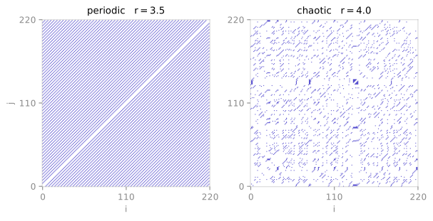
The plot tells periodic from chaotic at a glance. A periodic orbit recurs on long, clean, evenly spaced diagonals; deterministic chaos shatters them into a short-lined speckle — the visible signature the RQA measures below make numeric.

At a matched recurrence rate the logistic map's recurrence plot separates the regimes: a period-4 cycle ($r = 3.5$) recurs on clean parallel diagonals, while deterministic chaos ($r = 4.0$) breaks them into a short-lined speckle.

The radius \(\varepsilon\) is set one of two mutually-exclusive ways — pass exactly one of threshold= or recurrence_rate=:

Fixed radiusTarget recurrence rate

rm = ts.recurrence_matrix(x, threshold=0.05)   # ε = 0.05 in state units

A literal distance in the embedding's own units — direct, but the resulting recurrence rate then depends on the attractor's diameter, so it is not comparable across systems of different scale.

rm = ts.recurrence_matrix(x, recurrence_rate=0.05)   # pick ε so RR ≈ 5 %

recurrence_rate chooses \(\varepsilon\) from the empirical distribution of pairwise distances so the plot has the requested density. This is the scale-free, comparable choice — always prefer it when sweeping parameters or comparing systems, so that differences in the structure are not confounded with differences in the density.

metric selects the norm — "euclidean" (default), "manhattan", "chebyshev" (the maximum norm, the traditional RQA choice), or a numeric \(p\) for a general Minkowski distance. theiler=w blanks the central \(\pm w\) diagonals so that temporally-correlated neighbours along the line of identity are not mistaken for genuine recurrences (Theiler 1986); the default theiler=0 already drops the line of identity itself, and theiler=1 is a sensible minimum for a densely sampled flow.

The matrix is stored sparse

The recurrent pairs are found with a k-d tree range search (cKDTree.query_pairs), so a long series never materialises the dense \(N \times N\) array. rm.recurrence_rate reads the stored density directly; call rm.toarray() only when you genuinely need the dense boolean image.

Quantification: rqa

rqa reduces a recurrence matrix to the standard scalar measures of its diagonal and vertical line structure. Diagonal lines mark stretches where two trajectory segments evolve in parallel — the signature of deterministic dynamics; vertical lines mark states the system is trapped near for a while — the signature of laminar / intermittent phases. You can pass the same input as recurrence_matrix (a series or trajectory, with the same threshold / recurrence_rate / metric / theiler arguments) or a prebuilt RecurrenceMatrix.

x = ts.systems.Logistic(params={"r": 4.0}).iterate(steps=2000, ic=[0.4]).y[:, 0]
res = ts.rqa(x, recurrence_rate=0.05, theiler=1)

res.recurrence_rate      # ≈ 0.0496   RR — realised matrix density
res.determinism          # ≈ 0.652    DET — fraction of points on diagonals ≥ 2
res.laminarity           # ≈ 0.175    LAM — fraction of points on verticals ≥ 2
res.max_diagonal_length  # 17         L_max — longest diagonal (excl. the LOI)
res.divergence           # ≈ 0.0588   DIV = 1 / L_max
res.diagonal_entropy     # ≈ 1.358    ENTR — Shannon entropy of diagonal lengths
res.trapping_time        # ≈ 2.929    TT — mean vertical length

Field	Symbol	Meaning
recurrence_rate	RR	density of recurrence points
determinism	DET	fraction of points forming diagonal lines — predictability
laminarity	LAM	fraction forming vertical lines — intermittency / laminar phases
avg_diagonal_length	L	mean diagonal length
max_diagonal_length	L_max	longest diagonal — inversely related to the largest exponent
divergence	DIV	\(1/\mathrm{L}_{\max}\)
diagonal_entropy	ENTR	Shannon entropy (nats) of the diagonal-length histogram
trapping_time	TT	mean vertical length
max_vertical_length	V_max	longest vertical

min_diagonal / min_vertical set the shortest run counted as a line (default \(2\)) for the ratio and mean measures (DET / LAM / L / TT / ENTR); the maxima L_max / V_max are always the longest line in the unfiltered histogram (Marwan et al. 2007), and DIV = 1 / L_max. The raw run-length histograms survive on res.diagonal_lengths / res.vertical_lengths if you want to fit them yourself.

DET separates order from chaos

A periodic orbit recurs on perfectly parallel diagonals, so \(\mathrm{DET} = 1\); deterministic chaos breaks them up. Verified here: the logistic map at \(r = 3.2\) (a period-2 cycle) gives \(\mathrm{DET} = 1.0\) and \(\mathrm{LAM} = 0.0\), while the fully chaotic \(r = 4\) gives \(\mathrm{DET} \approx 0.65\) — squarely in the band Trulla, Giuliani, Zbilut & Webber (1996) report for that map.

Tracking regime change

The whole point of RQA is that it is local. windowed_rqa slides a window of window samples (advancing by step, default = window for non-overlapping windows) and runs rqa in each — so every measure becomes a time series that steps up or down as the dynamics cross between regimes. Each scalar RQA field is exposed as a per-window array aligned to wr.centers (the window-centre sample indices).

import numpy as np

# a series that is periodic for its first half, then switches to chaos
periodic = ts.systems.Logistic(params={"r": 3.5}).trajectory(1500, transient=500, ic=[0.2]).y[:, 0]
chaotic  = ts.systems.Logistic(params={"r": 4.0}).trajectory(1500, transient=500, ic=[0.4]).y[:, 0]
x = np.concatenate([periodic, chaotic])          # the switch is at sample 1500

wr = ts.windowed_rqa(x, window=300, step=150, recurrence_rate=0.05, theiler=1)

wr.centers        # window mid-points (the time axis)
wr.determinism    # DET(t): 1.0 through the periodic half, ≈ 0.65 in the chaotic half

wr.determinism — or any measure by name, wr.measure("laminarity") — reads \(1.0\) across every window inside the periodic segment and drops to \(\approx 0.65\) the moment the window enters the chaotic segment, pinning the transition to the window straddling sample \(1500\). wr.results is the tuple of per-window RQAResult objects if you need every field at once.

Choose window to span the dynamics

The window must be long enough to contain several recurrences yet short enough to be locally stationary. Too short and the line statistics are noisy; too long and a transition smears across windows. Size it from the system's characteristic period, and keep recurrence_rate fixed across windows so the measures stay comparable (the threshold is re-derived per window, so structure — not density — is what changes).

See also

• Lyapunov spectra — \(\mathrm{DIV} = 1/\mathrm{L}_{\max}\) tracks the largest exponent
• Chaos indicators — GALI, the 0–1 test, and expansion entropy: complementary chaos verdicts
• Surrogates & nonlinearity tests — test whether the recurrence structure is genuinely nonlinear
• Delay embedding — reconstruct a phase space before building the plot

References

• J.-P. Eckmann, S. O. Kamphorst and D. Ruelle, "Recurrence plots of dynamical systems", Europhys. Lett. 4, 973 (1987).
• J. Theiler, "Spurious dimension from correlation algorithms applied to limited time-series data", Phys. Rev. A 34, 2427 (1986).
• J. P. Zbilut and C. L. Webber, "Embeddings and delays as derived from quantification of recurrence plots", Phys. Lett. A 171, 199 (1992).
• L. L. Trulla, A. Giuliani, J. P. Zbilut and C. L. Webber, "Recurrence quantification analysis of the logistic equation with transients", Phys. Lett. A 223, 255 (1996).
• N. Marwan, M. C. Romano, M. Thiel and J. Kurths, "Recurrence plots for the analysis of complex systems", Phys. Rep. 438, 237 (2007).