Analysis · Integration & methods

Integration & methods

Every system in the catalogue advances the same way. You call one verb, the library lowers the symbolic dynamics to an in-process tape, and the Rust engine marches it. This page is the practical guide to that march: which verb to call, what the resulting Trajectory gives you, how to pick a solver, what automatic stiffness selection does, and which backend runs the numbers — followed by the complete capability table of every solver in the registry.

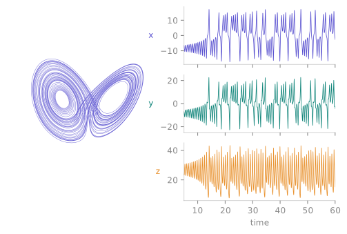
One Lorenz().integrate(...) call returns one Trajectory. The same data is the strange attractor in state space (left, indigo) and the stacked x(t), y(t), z(t) time series it samples on the output grid (right) — traj.y is (T, dim), traj["x"] is one column of it.

Two verbs: integrate and iterate

Continuous families (ODEs, DDEs, SDEs) integrate; discrete maps iterate. Both return a single Trajectory.

import tsdynamics as ts

# flows — integrate over a time span, sampled on an output grid
traj = ts.systems.Lorenz().integrate(final_time=100.0, dt=0.01)

# maps — iterate a fixed number of steps
orbit = ts.systems.Henon().iterate(steps=10_000)

For a flow there are two grids in play. The internal steps — chosen by the solver to meet rtol/atol — decide accuracy; the output grid dt only decides where the solution is sampled into the returned arrays. A coarse dt loses resolution, never accuracy. (Fixed-step kernels are the exception: there dt is the integration step.)

The Trajectory object

Every integrate or iterate call returns a Trajectory: time points t of shape (T,), states y of shape (T, dim), and provenance. It is the lingua franca of the whole toolkit — every quantifier accepts one, and every derived wrapper produces one.

traj.t, traj.y               # the arrays: (T,) and (T, dim)
traj.dim, traj.n_steps       # 3, 10001
t, y = traj                  # tuple-unpacking compatibility

traj["x"]                    # named component → (T,)   (needs class `variables`)
traj[["x", "z"]]             # multiple components → (T, 2)
traj[100:200]                # row slicing → new Trajectory (t and y together)
traj.component(2)            # by index

traj.after(20.0)             # drop the transient: keep t >= 20
traj.minmax()                # per-component (minima, maxima)
traj.standardize()           # zero mean, unit std per component (records the transform)
traj.neighbors(q, k=3)       # (distances, indices) of the k nearest points to q (cached KD-tree)

Slicing keeps t and y together and preserves the metadata, so a transient-dropped or windowed trajectory is still a fully self-describing Trajectory. traj.meta carries the provenance — the system name, a snapshot of the parameters, the solver, the tolerances, the backend, and the actual initial condition used:

traj.meta
# {'system': 'Lorenz', 'params': {...}, 'tsdynamics': '5.2.6', 'engine': 'rust',
#  'family': 'ode', 'method': 'rk45', 'backend': 'interp', 'dt': 0.01, 't0': 0.0,
#  'rtol': 1e-06, 'atol': 1e-09, 'ic': array([...])}

A result you cannot trace is a result you cannot reproduce; the snapshot makes every saved trajectory self-describing.

The stepping API

integrate / iterate produce whole trajectories in one call. For algorithms that need control — advance a little, look at the state, decide, advance again — every system also implements the incremental System protocol:

lor = ts.systems.Lorenz()
lor.reinit([1.0, 1.0, 1.0])      # explicit start (optional — step() lazily reinits)
u = lor.step(0.01)               # advance dt=0.01, get the new state
lor.state(), lor.time()          # current state / time
lor.set_state(u + 1e-9)          # overwrite the state in place

• step(n_or_dt) — a number of iterations for maps (default 1), a time increment for flows (default 0.01 for ODEs, 0.1 for DDEs). Returns the new state.
• reinit(u, *, t=..., params=...) — restart the internal stepper; parameter overrides are applied first.
• state() / time() / set_state(u) — read the live state and time, or overwrite the state in place.
• trajectory(...) — a protocol-uniform wrapper over integrate / iterate with a transient= drop.

set_state on a DDE raises — by design

A delay system's instantaneous state is a history function over \([t - \tau_{\max},\, t]\), not a point, so overwriting it with a single vector is not meaningful. DelaySystem.set_state raises NotImplementedError; use reinit(u) to restart from a constant past instead. This is also why max_lyapunov (which needs set_state) excludes DDEs.

The protocol is what the rest of the toolkit is written against — orbit diagrams, Poincaré maps and max_lyapunov are all loops over step(). When a prepackaged analysis does not fit, you drive it directly; see the Analysis toolkit.

Choosing a solver

The method= keyword selects the integration kernel. The default is rk45 (Dormand–Prince 5(4)), a robust general-purpose adaptive explicit solver that serves most non-stiff systems well.

traj = sys.integrate(final_time=100.0, dt=0.02, method="dop853", rtol=1e-9, atol=1e-12)

There are three broad regimes:

• Fixed-step explicit (euler, rk4, ssprk3, …) — no error control; the step is dt. Cheap and fully deterministic, the right choice when you want an exact, reproducible discretisation (the Poincaré crossing march and the three.js viewers integrate on a fixed-step rk4 for this reason). The trade-off is that you own the step: too coarse and the orbit drifts.
• Adaptive explicit (rk45, tsit5, dop853, …) — embedded error estimators shrink and grow the internal step to hold rtol/atol. The default regime for smooth, non-stiff dynamics. Reach for dop853 when you need high accuracy at tight tolerances (e.g. reference Lyapunov runs).
• Implicit / stiff (bdf, rosenbrock, trbdf2, …) — solve a (possibly nonlinear) system each step using the Jacobian, so they stay stable on stiff problems where an explicit kernel would need a punishingly small step. bdf (variable-order 1–5) is the recommended stiff default. The engine builds the Jacobian-carrying tape automatically for these kernels — method="bdf" just works, no hand-written Jacobian required.

A system that is known to be stiff should declare _default_method = "bdf" on its class, so it picks the right kernel without the caller having to know. Several catalogue systems already do (e.g. KuramotoSivashinsky, Duffing).

Tolerances tune accuracy, not the output grid

rtol / atol govern the internal adaptive steps. Tightening them refines the path the solver actually traces; it does not change where the result is sampled. To sample more densely, shrink dt. DDEs start from looser defaults (rtol = atol = 1e-3) — delay systems are sensitive, and that is the safe starting point.

Automatic stiffness selection

If you do not know whether a system is stiff, ask the library to find out:

traj = sys.integrate(final_time=100.0, dt=0.02, method="auto")
traj.meta["method"]    # the kernel that was actually used, e.g. "rk45" or "bdf"

method="auto" lowers the problem, probes the Jacobian spectrum at the start state with the one-point solvers.recommend heuristic, and selects bdf on a stiff right-hand side or rk45 otherwise. The resolved kernel is recorded in traj.meta["method"], so the choice is always visible after the fact. It is honoured consistently across every entry point — integrate, ensemble, the resumable stepping protocol, and the events seam.

Because the probe is taken at a single point, it is initial-condition dependent: it is a convenience, not an oracle. A system you know to be reliably stiff should still declare _default_method = "bdf" rather than lean on "auto". For maps, which have no solver kernel, "auto" is a harmless no-op.

Backends: interp, jit, reference

Orthogonal to which solver runs is what executes it. The same method= runs on any of three backends, selected with backend=:

backend	What it is	When to use it
"interp"	The Rust SSA-tape interpreter (the default)	Everyday integration — no warmup, no compile step
"jit"	The Cranelift JIT — compiles the tape to native code	Long or repeated runs where the per-step compiled speed pays for itself; bit-for-bit identical results to interp
"reference"	A dependency-light pure-Python SciPy oracle (ODEs + maps)	Cross-validation and wheel-free environments — the answer key, not the fast path

traj = sys.integrate(final_time=100.0, dt=0.01, backend="jit")

interp and jit lower the same tape, so they agree bit-for-bit; reference is an independent implementation kept as a correctness oracle. Not every family supports reference — DDEs have no pure-Python integrator and reject it loudly rather than silently degrading.

Solver capability table

Every solver lives in the solver registry — a name → SolverSpec table with capability flags. The table below is the complete registry, generated directly from tsdynamics.solvers.all_specs(). Each method= string accepted by integrate is one row here. (The name column is the exact method= value; common aliases such as "RK45" / "dopri5" resolve to rk45.)

Explicit · fixed-step

method	Kind	Adaptive	Needs Jacobian	Family	Description	Origin
euler	explicit	—	—	ode	forward (explicit) Euler (order 1, fixed step)	builtin
midpoint	explicit	—	—	ode	explicit midpoint / modified Euler (order 2, fixed step)	builtin
heun	explicit	—	—	ode	Heun's method / explicit trapezoid (order 2, fixed step)	builtin
ralston	explicit	—	—	ode	Ralston's minimum-error-bound RK2 (order 2, fixed step)	builtin
rk4	explicit	—	—	ode	classic 4th-order Runge–Kutta (fixed step)	builtin
rk4_38	explicit	—	—	ode	the 3/8-rule 4th-order Runge–Kutta (fixed step)	builtin
ssprk3	explicit	—	—	ode	3rd-order strong-stability-preserving RK (Shu–Osher, fixed step)	builtin
ab3	explicit	—	—	ode	Adams–Bashforth 3-step explicit multistep (order 3)	builtin
ab4	explicit	—	—	ode	Adams–Bashforth 4-step explicit multistep (order 4)	builtin
abm4	explicit	—	—	ode	Adams–Bashforth–Moulton predictor–corrector (PECE, order 4)	builtin

Explicit · adaptive

method	Kind	Adaptive	Needs Jacobian	Family	Description	Origin
heun_euler	explicit	yes	—	ode	Heun–Euler 2(1) adaptive	builtin
bs3	explicit	yes	—	ode	Bogacki–Shampine 3(2) adaptive (ode23)	builtin
rk45	explicit	yes	—	ode	Dormand–Prince 5(4) adaptive (dopri5)	builtin
rkf45	explicit	yes	—	ode	Runge–Kutta–Fehlberg 4(5) adaptive	builtin
cashkarp	explicit	yes	—	ode	Cash–Karp 5(4) adaptive	builtin
tsit5	explicit	yes	—	ode	Tsitouras 5(4) adaptive	builtin
dop853	explicit	yes	—	ode	Dormand–Prince 8(5,3) adaptive	builtin

Implicit / stiff

These solve a system each step using the Jacobian (needs_jacobian = yes); the engine lowers the Jacobian-carrying tape automatically.

method	Kind	Adaptive	Needs Jacobian	Family	Description	Origin
backward_euler	implicit	yes	yes	ode	implicit (backward) Euler (order 1, L-stable)	builtin
implicit_midpoint	implicit	yes	yes	ode	implicit midpoint rule / 1-stage Gauss (order 2, A-stable)	builtin
trapezoid	implicit	yes	yes	ode	implicit trapezoidal rule / Crank–Nicolson (order 2, A-stable)	builtin
sdirk2	implicit	yes	yes	ode	2-stage L-stable SDIRK (Alexander, order 2)	builtin
rosenbrock	implicit	yes	yes	ode	linearly-implicit Rosenbrock-W (one linear solve per step)	builtin
trbdf2	implicit	yes	yes	ode	TR-BDF2 composite ESDIRK (trapezoidal + BDF2)	builtin
bdf	implicit	yes	yes	ode	variable-order (1–5) fixed-leading-coefficient BDF	builtin

Stochastic (SDE)

Fixed-step schemes for diagonal-Itô SDEs. Here dt sets both the discretisation and the noise scale \(\sqrt{dt}\).

method	Kind	Adaptive	Needs Jacobian	Family	Description	Origin
euler_maruyama	explicit	—	—	sde	Euler–Maruyama diagonal-Itô (strong order 0.5)	builtin
milstein	explicit	—	yes	sde	Milstein diagonal-Itô (strong order 1.0; uses ∂g/∂u)	builtin

Why there is no order or stability column

A SolverSpec carries only the capability flags shown above — kind, adaptive, needs_jacobian, and the supported family. It has no structured order or stability field, so this table does not fabricate one: a kernel's order and stability region are stated in its prose description, sourced from the original literature, rather than reduced to a column the registry cannot back.

Self-documenting solvers

The registry is the single source of truth. Any solver — built-in or shipped by a plugin — appears in solvers.all_specs() with its capability flags and description, which is exactly what this table renders. A new kernel registered through the solver registry therefore documents itself: it becomes selectable by method= and shows up here on the next docs build, with no separate documentation step. The origin column distinguishes registry-builtin kernels from out-of-tree contributions; today every solver is builtin.

See also

• Analysis toolkit — the Trajectory object, the stepping protocol, and the quantifiers
• Systems — the 171 built-in systems you can integrate