Analysis · Surrogates

Surrogates & nonlinearity tests¶

Before you fit a Lyapunov exponent or a fractal dimension to a measured series, there is a prior question worth answering: can the structure in this series be explained by a linear stochastic process? If a linear Gaussian model (possibly seen through a static nonlinear measurement) already accounts for everything you observe, the fancy nonlinear quantifiers are measuring noise. The surrogate- data method turns that into a hypothesis test: generate an ensemble of surrogates that reproduce the chosen linear properties of the data — its amplitude distribution and/or its power spectrum — but are otherwise random, compute a discriminating statistic on the data and on each surrogate, and reject the linear null when the data sits in the tail of the surrogate distribution (Theiler, Eubank, Longtin, Galdrikian & Farmer 1992).

Function	Builds / does	Preserves
`random_shuffle`	a random permutation of the samples	amplitude distribution only
`fourier_surrogate`	randomised Fourier phases	power spectrum (linear autocorrelation)
`aaft_surrogate`	amplitude-adjusted FT	distribution and spectrum
`iaaft_surrogate`	iterative AAFT	distribution + spectrum, refined
`surrogate_test`	the ensemble test → `SurrogateTest`	rank-based $p$ and a $z$-score

The test¶

surrogate_test is the one-call entry point: it draws the surrogates, scores the data against them with a nonlinearity-sensitive statistic, and returns a SurrogateTest carrying a rank-based $p$-value, a $z$-score (the data statistic's distance from the null mean, in surrogate standard deviations), and the boolean verdict rejected (true when $p \le$ alpha).

import tsdynamics as ts

# Lorenz z — the discriminating observable for a time-reversal test
z = ts.Lorenz().trajectory(final_time=150.0, dt=0.05, transient=20.0,
                           ic=[1.0, 1.0, 1.0])["z"]

res = ts.surrogate_test(z, statistic="time_reversal",
                        method="iaaft", n=200, seed=0)

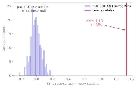
res.data_statistic   # ≈ 1.13   asymmetry of the real data
res.p_value          # ≈ 0.01   as extreme as the ensemble allows
res.z_score          # ≈ 18.6   sigmas above the null mean
res.rejected         # True     → linear-stochastic null rejected

A dissipative chaotic flow is strongly time-irreversible, whereas every linear-Gaussian null (and any static nonlinear rescaling of one) is time-symmetric — so the data statistic lands far outside the surrogate histogram, and the null is rejected.

IAAFT surrogate null distribution of the time-reversal statistic with the Lorenz-z data value far in the tail — A surrogate test of the Lorenz $z$-component: the time-reversal-asymmetry statistic on the data (rose) sits $\approx 18.6\,\sigma$ outside the null distribution of 200 IAAFT surrogates (indigo), so the linear-stochastic null is rejected at $p \approx 0.01$.

The surrogate count defaults to n=39, which follows Theiler's rule $M = 2/\alpha - 1$ for a two-sided test at $\alpha = 0.05$ — the smallest ensemble whose most-extreme attainable rank gives an exact nominal level. Raising n (200 in the figure) sharpens the null histogram and lowers the smallest reachable $p$. method= selects the generator ("iaaft" default), tail="auto" picks the rejection side from the statistic, and seed= fixes the surrogate draw so the whole test is reproducible.

The complement is just as important — a genuinely linear process should pass the test:

import numpy as np

rng = np.random.default_rng(0)
ar = np.zeros(2000)
for i in range(1, 2000):                       # AR(1), φ = 0.5 — linear Gaussian
    ar[i] = 0.5 * ar[i - 1] + rng.standard_normal()

ts.surrogate_test(ar, statistic="time_reversal", n=39, seed=1).rejected   # False

Over many seeds the AR(1) false-positive rate sits at the nominal $\alpha$ (≈ 0.05) — exactly what an honest test must deliver on data that really is linear. A test that "rejects everything" is not detecting nonlinearity; it is broken.

Generators¶

Each generator returns an array of shape (n, N) — n surrogates of the length-N input — and is fully seed-reproducible. They differ in which linear fingerprint they preserve, and therefore in which null they realise:

x = ts.systems.Logistic(params={"r": 4.0}).trajectory(2000, transient=500, ic=[0.1]).y[:, 0]

ts.iaaft_surrogate(x, n=5, seed=1).shape       # (5, 2000)
ts.fourier_surrogate(x, n=39, seed=1)          # phase-randomised, spectrum kept
ts.random_shuffle(x, n=39, seed=1)             # only the value histogram kept

random_shuffle — a random permutation of the samples. Keeps the amplitude histogram exactly and destroys every temporal correlation: the null of an i.i.d. process ("are successive samples even dependent?").
fourier_surrogate — randomises the Fourier phases, so the magnitude (and hence power) spectrum and the linear autocorrelation are preserved exactly while any phase coupling is erased. The null of a stationary linear Gaussian process. Its amplitude distribution drifts toward Gaussian — use the AAFT family when the distribution must be kept too.
aaft_surrogate / iaaft_surrogate — preserve both the amplitude distribution and the spectrum, realising the null of a static monotonic nonlinearity acting on a linear Gaussian process. The iterative variant alternately rescales in the spectral and amplitude domains to remove the small spectral bias plain AAFT leaves behind (Schreiber & Schmitz 1996), and is the recommended default.

You rarely call these directly — surrogate_test(..., method=...) does — but they are public, and ts.surrogates(x, method, n, seed=...) is the by-name dispatcher (returning a SurrogateEnsemble that behaves as the (n, N) array) for building bespoke tests or diagnostics.

Statistics¶

The discriminating statistic must be sensitive to nonlinearity yet blind to the linear structure the surrogates preserve — otherwise it would flag the surrogates too. Both shipped choices meet that bar:

ts.time_reversal_asymmetry(x)              # ≈ -0.724 for logistic r = 4
ts.nonlinear_prediction_error(x, dimension=3, delay=1, horizon=1, n_neighbors=4)

time_reversal_asymmetry — the dimensionless third-moment ratio of the lagged increments,

$$ T_\text{rev} \;=\; \frac{\langle (x_{t} - x_{t-\ell})^3 \rangle} {\langle (x_{t} - x_{t-\ell})^2 \rangle^{3/2}}, $$

which changes sign under time reversal and is therefore zero in expectation for any time-reversible process — every linear Gaussian process and every static monotonic transform of one. Nonzero asymmetry is a hallmark of nonlinearity; it is a cheap, robust default (Schreiber & Schmitz 1996; Diks et al. 1995). - nonlinear_prediction_error — the out-of-sample error of a locally-constant predictor in a delay embedding (Sugihara & May 1990; Kantz & Schreiber 2004), normalised so an unpredictable series scores $\approx 1$. Deterministic data is more predictable than its phase-randomised surrogates, so this is the one-sided tail="less" statistic — surrogate_test infers that automatically:

x = ts.systems.Logistic(params={"r": 4.0}).trajectory(2000, transient=500, ic=[0.1]).y[:, 0]
res = ts.surrogate_test(x, statistic="prediction_error", n=39, seed=1)
res.p_value, res.rejected     # ≈ 0.025, True   → linear null rejected
res.z_score                   # ≈ -101  (data far more predictable than surrogates)

Pick the discriminating observable

A multivariate series is reduced to one channel (component=, default the highest-variance one). The right observable matters. For the Lorenz system the $x$ and $y$ components are nearly time-symmetric, so a time-reversal test on them rejects only weakly (0/10 and 2/10 seeds in the validation suite) — the $z$ component is the discriminating observable and rejects the linear null on 10/10 seeds. Choose the observable that the nonlinearity actually lives in.

The result record¶

res = ts.surrogate_test(z, n=39, seed=1)
res.data_statistic          # statistic on the data
res.surrogate_statistics    # array of the n surrogate statistics (the null)
res.p_value, res.z_score    # rank-based p; (data − mean)/std in σ units
res.rejected                # p_value <= alpha
res.statistic, res.method, res.tail, res.alpha, res.n_surrogates

SurrogateTest is an AnalysisResult, so it carries .meta, .summary(), .to_dict(), and a .plot seam that renders the null histogram with the data value marked and the rejection tail shaded.

A surrogate test never proves nonlinearity

Rejecting the linear null only says the chosen surrogates' linear properties cannot account for the statistic — it does not identify which nonlinearity, nor rule out non-stationarity or a poorly matched null. Match the generator to the property you want to control for, prefer IAAFT when the distribution is non-Gaussian, and always report the statistic and method alongside the verdict.

References¶

J. Theiler, S. Eubank, A. Longtin, B. Galdrikian and J. D. Farmer, "Testing for nonlinearity in time series: the method of surrogate data", Physica D 58, 77 (1992).
T. Schreiber and A. Schmitz, "Improved surrogate data for nonlinearity tests", Phys. Rev. Lett. 77, 635 (1996).
C. Diks, J. C. van Houwelingen, F. Takens and J. DeGoede, "Reversibility as a criterion for discriminating time series", Phys. Lett. A 201, 221 (1995).
G. Sugihara and R. M. May, "Nonlinear forecasting as a way of distinguishing chaos from measurement error in time series", Nature 344, 734 (1990).
H. Kantz and T. Schreiber, Nonlinear Time Series Analysis, 2nd ed., Cambridge University Press (2004).