Analysis · Entropy & complexity

Entropy & complexity

How unpredictable is a signal? Entropy measures answer that without a model of the dynamics — from a single measured series they quantify how much new information each sample carries, distinguishing periodic order from deterministic chaos from stochastic noise. TSDynamics ships the standard family (permutation, dispersion, sample, approximate, multiscale, and Lempel–Ziv) and — the design that ties them together — a composable core that builds any of them from three orthogonal choices.

Every scalar entropy reads a 1-D array, a 2-D array (with component=), or a Trajectory (with component= naming a variable), so they consume the trajectory lingua franca directly. The named measures live under tsdynamics.analysis.entropy:

from tsdynamics.analysis.entropy import (
    permutation_entropy, weighted_permutation_entropy,
    dispersion_entropy, sample_entropy, approximate_entropy,
    multiscale_entropy, lz76_complexity, lz76_entropy,
)

The composable core

An entropy estimate of a time series is three independent decisions stacked on top of one another:

1. an outcome space — how a real-valued series is turned into a finite set of discrete symbols and counted (ordinal patterns, dispersion patterns, amplitude bins, raw symbols);
2. a probability estimator — how outcome counts become a probability vector (maximum likelihood / relative frequency, or additive smoothing for short series);
3. an information measure — the functional applied to that vector (Shannon, Rényi, or Tsallis).

entropy(...) composes the three; every named function below is a thin wrapper that fixes the outcome space. Building an estimator explicitly makes the choices visible — and lets you mix combinations the named wrappers do not expose:

import numpy as np
from tsdynamics.analysis.entropy import (
    entropy, OrdinalPatterns, Dispersion, AmplitudeBinning,
    MLE, AddConstant, Shannon, Renyi, Tsallis,
)

noise = np.random.default_rng(0).standard_normal(5000)

# Shannon entropy of ordinal (permutation) patterns — this IS permutation_entropy
entropy(noise, outcomes=OrdinalPatterns(m=4), measure=Shannon(base=2),
        normalize=True)                                    # 0.999

# swap in the Rényi (order q=2) measure over the same outcome space
entropy(noise, outcomes=OrdinalPatterns(m=3), measure=Renyi(q=2.0),
        normalize=True)                                    # 1.000

# Laplace-smoothed dispersion patterns for a short series (regularises zeros)
entropy(noise[:200], outcomes=Dispersion(c=6, m=2), prob=AddConstant(a=1.0),
        normalize=True)                                    # 0.993

With normalize=True the result is divided by the measure's maximum over the outcome alphabet, mapping it to \([0, 1]\): 0 for a perfectly ordered signal, 1 for uniform symbol usage. probabilities(x, outcomes) returns the raw outcome distribution if you want to plot or reuse it.

Permutation entropy

The most widely used ordinal measure (Bandt & Pompe 2002). Each length-\(m\) window is encoded by the permutation that sorts it — its ordinal pattern — and the Shannon entropy of the pattern distribution is the permutation entropy. It depends only on the relative rankings of samples, so it is invariant under any strictly monotonic transform of the data and needs no amplitude thresholds, which makes it robust for noisy experimental series.

import tsdynamics as ts

logistic = ts.systems.Logistic(params={"r": 4.0})
chaotic = logistic.iterate(steps=5000, ic=[0.1234]).y[500:, 0]

permutation_entropy(chaotic, dimension=4)                 # 0.742  (chaos)
permutation_entropy(np.random.default_rng(0).standard_normal(5000),
                    dimension=4)                          # 0.999  (noise)
permutation_entropy(np.sin(np.linspace(0, 50 * np.pi, 5000)),
                    dimension=4)                          # 0.258  (periodic)
permutation_entropy(np.arange(1000.0))                    # 0.000  (monotone)

weighted_permutation_entropy restores sensitivity to amplitude — each pattern is weighted by the variance of its window, so abrupt large-amplitude events count more than tiny fluctuations sharing the same ordinal pattern (Fadlallah et al. 2013).

Dispersion entropy

Where permutation entropy discards amplitude, dispersion entropy keeps it (Rostaghi & Azami 2016). The series is mapped through the normal CDF onto \(c\) amplitude classes, embedded with order \(m\), and the Shannon entropy of the resulting dispersion patterns over the \(c^m\) alphabet is returned. It is markedly faster than sample entropy while staying robust to noise:

dispersion_entropy(noise, c=6, dimension=2)               # 0.999

White noise normalises to slightly below 1 at finite length

With normalize=True the entropy is divided by \(\log_b(c^m)\), the log of the full dispersion-pattern alphabet (the canonical Rostaghi & Azami convention). A finite series can populate at most \(n - (m-1)\tau\) of those \(c^m\) patterns, so even ideal white noise sits just under 1 — approaching it only as \(n \to \infty\). This is expected, not a defect.

Sample & approximate entropy

These are correlation-integral statistics rather than members of the outcome-space family: they count how often short template windows recur within a tolerance \(r\), and are reported in nats.

Sample entropy (Richman & Moorman 2000) is \(\text{SampEn} = -\ln(A/B)\), where \(B\) and \(A\) count template pairs (excluding self-matches) that stay within Chebyshev tolerance \(r\) over windows of length \(m\) and \(m+1\). Excluding self-matches removes the length bias of the older approximate entropy, making the statistic largely independent of series length:

sample_entropy(noise)                                     # 2.206  (irregular)
sample_entropy(np.sin(np.linspace(0, 50 * np.pi, 5000)))  # 0.074  (regular)

The default tolerance is \(r = 0.2\,\sigma\). approximate_entropy (Pincus 1991) is the earlier, self-matching variant — prefer sample entropy when its downward short-series bias matters.

Multiscale entropy

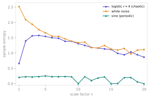
A single-scale entropy cannot tell a \(1/f\)-correlated process from white noise — both look highly irregular at the finest scale. Multiscale entropy (Costa et al. 2002) resolves this by measuring an entropy on coarse-grained copies of the series: for each scale factor the series is split into non-overlapping windows of that length and each replaced by its mean, then the entropy is recomputed. The shape of the resulting curve is the discriminator.

mse_chaotic = ts.multiscale_entropy(chaotic, scales=20)
mse_noise = ts.multiscale_entropy(noise, scales=20)

mse_noise[0] > mse_noise[-1]   # True — uncorrelated noise decays with scale

White noise starts high and decays as coarse-graining averages away its uncorrelated fine structure; a structured signal with correlations across scales holds a roughly flat (or rising) profile. The figure contrasts three canonical cases at matched settings: chaotic logistic (\(r=4\)), white noise, and a smooth sine.

Following Costa et al., when the chosen entropy takes a tolerance \(r\) it is fixed across all scales from the original series' standard deviation (default \(r = 0.15\,\sigma\)), so the profile reflects structure rather than the shrinking variance of the coarse-grained signal. Any of this package's scalar entropies can drive it via entropy_fn=.

FIG 1 · multiscale sample entropy vs scale factor. White noise (amber) decays with scale; the chaotic logistic map (indigo) holds high complexity across scales; the periodic sine (teal) stays near zero.

Lempel–Ziv complexity

The LZ76 complexity \(c(S)\) of a symbol sequence is the number of factors in its exhaustive-history parse — each factor a substring not seen before (Lempel & Ziv 1976; Kaspar & Schuster 1987). It is a threshold-free structural measure: a periodic sequence parses into few factors, an incompressible one into many. The normalised density \(h \approx c(S)\,\log_k(n)/n\) (with \(k\) the alphabet size) converges to the source entropy rate, so LZ76 doubles as a fast entropy estimator.

Continuous signals are symbolised first — median-threshold binarisation is the standard choice — while strings and integer arrays are treated as already symbolic:

lz76_complexity("0001101001000101", symbolize=None)      # 6.0  (Kaspar–Schuster)
lz76_complexity("aaaaaaaa", symbolize=None)               # 2.0  (constant)

lz76_entropy(noise)                                       # 1.037  (irregular)
lz76_entropy(np.sin(np.linspace(0, 50 * np.pi, 5000)))    # 0.012  (periodic)

lz76_entropy(x) is lz76_complexity(x, normalize=True); lz76_factors returns the factor-boundary indices if you want to inspect the parse.

Different measures, different questions

These estimators are not interchangeable numbers. Permutation entropy is ordinal and monotone-invariant; dispersion and weighted-permutation entropy restore amplitude; sample entropy measures template recurrence; LZ76 measures compressibility. They agree on the qualitative ranking (periodic < chaotic < random) but not on absolute values — the "regular vs random" ordering is the robust signal, and TSDynamics' own test suite checks that five independent complexity measures concur on it.

Choosing a measure

You want…	Reach for	Why
A fast, robust, threshold-free default	permutation_entropy	ordinal, monotone-invariant, noise-tolerant
Amplitude sensitivity kept	dispersion_entropy, weighted_permutation_entropy	encode magnitude, not just rank
The physiologic / template-recurrence standard	sample_entropy	length-bias-free correlation integral
To separate correlated structure from noise	multiscale_entropy	the shape across scales discriminates
A model-free compressibility / entropy-rate estimate	lz76_complexity / lz76_entropy	symbolic, threshold-free
A combination the wrappers don't expose	entropy(...)	compose outcome × estimator × measure

See also

• Fractal dimensions — a complementary, geometric view of the same complexity
• Recurrence & RQA — recurrence-based quantifiers of structure
• Surrogates — test whether a complexity value is significant against a stochastic null
• Delay embeddings — the reconstruction step ordinal-pattern and sample-entropy embeddings share

References

• C. Bandt and B. Pompe, "Permutation entropy: a natural complexity measure for time series", Phys. Rev. Lett. 88, 174102 (2002).
• B. Fadlallah, B. Chen, A. Keil and J. Príncipe, "Weighted-permutation entropy: a complexity measure for time series incorporating amplitude information", Phys. Rev. E 87, 022911 (2013).
• M. Rostaghi and H. Azami, "Dispersion entropy: a measure for time-series analysis", IEEE Signal Process. Lett. 23, 610 (2016).
• S. M. Pincus, "Approximate entropy as a measure of system complexity", Proc. Natl. Acad. Sci. USA 88, 2297 (1991).
• J. S. Richman and J. R. Moorman, "Physiological time-series analysis using approximate entropy and sample entropy", Am. J. Physiol. Heart Circ. Physiol. 278, H2039 (2000).
• M. Costa, A. L. Goldberger and C.-K. Peng, "Multiscale entropy analysis of complex physiologic time series", Phys. Rev. Lett. 89, 068102 (2002).
• A. Lempel and J. Ziv, "On the complexity of finite sequences", IEEE Trans. Inf. Theory 22, 75 (1976).
• F. Kaspar and H. G. Schuster, "Easily calculable measure for the complexity of spatiotemporal patterns", Phys. Rev. A 36, 842 (1987).