KuramotoSivashinsky

Systems · Continuous · Chaotic attractors

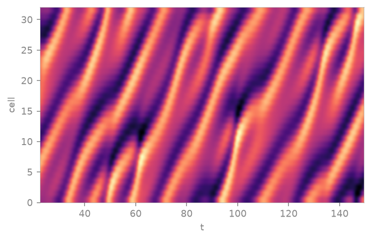
1D Kuramoto–Sivashinsky PDE on a periodic domain, discretized with N grid points.

Dimension: variable

Equations

@staticmethod
def _equations(Y, t, *, N, L):
    # 7-point central weights (Trefethen-style) for periodic, equispaced grid.
    # First derivative (6th-order): D1 * f / dx
    w1 = (
        -1.0 / 60.0,
        3.0 / 20.0,
        -3.0 / 4.0,
        0.0,
        3.0 / 4.0,
        -3.0 / 20.0,
        1.0 / 60.0,
    )
    # Second derivative (6th-order): D2 * f / dx^2
    w2 = (
        1.0 / 90.0,
        -3.0 / 20.0,
        3.0 / 2.0,
        -49.0 / 18.0,
        3.0 / 2.0,
        -3.0 / 20.0,
        1.0 / 90.0,
    )
    # Fourth derivative (7-point central): D4 * f / dx^4
    w4 = (-1.0 / 6.0, 2.0, -6.5, 28.0 / 3.0, -6.5, 2.0, -1.0 / 6.0)
    offsets = (-3, -2, -1, 0, 1, 2, 3)

    dx = L / N
    inv_dx = 1.0 / dx
    inv_dx2 = inv_dx * inv_dx
    inv_dx4 = inv_dx2 * inv_dx2

    rhs = []
    for j in range(N):
        # Nonlinear term: -u * u_x (structure-preserving)
        ux = 0.0
        for r, c in zip(offsets, w1, strict=True):
            idx = (j + r) % N
            ux += c * Y(idx)
        ux *= inv_dx

        nonlinear = -Y(j) * ux

        # u_xx: 6th-order central
        uxx = 0.0
        for r, c in zip(offsets, w2, strict=True):
            idx = (j + r) % N
            uxx += c * Y(idx)
        uxx *= inv_dx2

        # u_xxxx: 7-point central
        uxxxx = 0.0
        for r, c in zip(offsets, w4, strict=True):
            idx = (j + r) % N
            uxxxx += c * Y(idx)
        uxxxx *= inv_dx4

        rhs.append(nonlinear - uxx - uxxxx)
    return rhs

Parameters

parameter	default
N	32
L	22.0

Usage

import tsdynamics as ts

sys = ts.KuramotoSivashinsky()
traj = sys.integrate(final_time=100.0, dt=0.01)

Back to Chaotic attractors