Plotting

import numpy as np
import matplotlib.pyplot as plt
import hilbertplot as hp

t = np.arange(4096)
values = np.sin(2 * np.pi * t / 97) + 0.4 * np.cos(2 * np.pi * t / 31)
fig = hp.plot(values, curve=12)
plt.show()

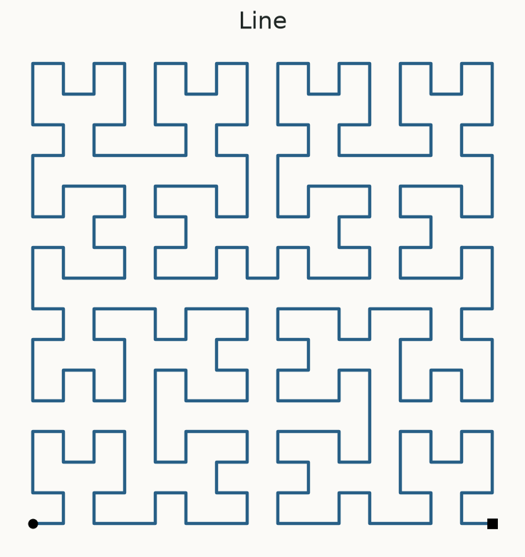
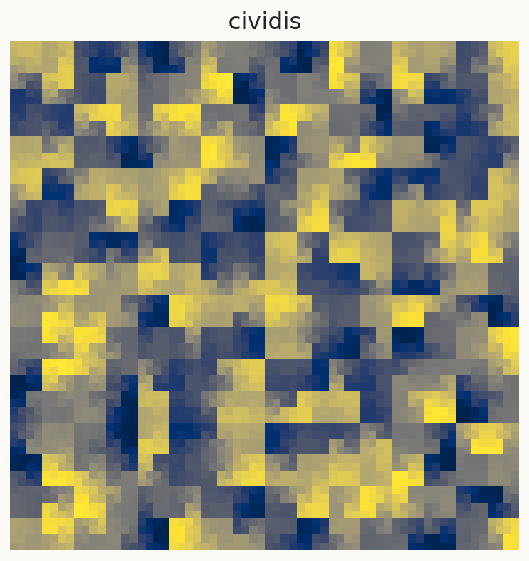
The curve walks through a square grid. Value values[i] goes into the i-th visited cell. A colour represents the value in that cell. Each call makes one plot.

Choose by number or label

hp.plot(values, curve=0)          # Hilbert, the default
hp.plot(values, curve="Moore")   # a named curve
hp.plot(values, curve="12H")     # a paper symbol

Every catalog entry has an index from 0 through 39. You never need to remember a generated label.

Save the figure

fig = hp.plot(values, curve=12)
fig.savefig("sequence.png", dpi=200)
fig.savefig("sequence.pdf")
plt.close(fig)

Drawing does not call plt.show() or close your figure. In scripts, call plt.show() after preparing the figures you want. In notebooks, the plotting backend normally displays them.

Colormaps

hp.plot(values, cmap="viridis")
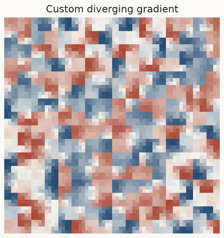
hp.plot(values, cmap=["navy", "white", "firebrick"], vmin=-1, vmax=1)

A colour list defines a smooth gradient: low values use its first colour, middle values pass through the intermediate colours, and high values use its last colour. It does not assign colours to categories.

Sequential: color increases across the full numeric range.

Diverging: zero is neutral; negative and positive values have different hues.

Custom gradient: the supplied colors are interpolation stops.

Color normalization

For positive values with a large dynamic range:

from matplotlib.colors import LogNorm

positive = np.exp(3 * np.sin(t / 37))
hp.plot(positive, cmap="inferno", norm=LogNorm(vmin=np.exp(-3), vmax=np.exp(3)))

Use either norm= or vmin/vmax. When passing a norm, put limits on the norm itself.

Use your own axes

fig, ax = plt.subplots()
hp.plot(values, curve=12, ax=ax, title="My sequence")

A colourbar is enabled by default. Pass colorbar=False to omit it.

Missing values

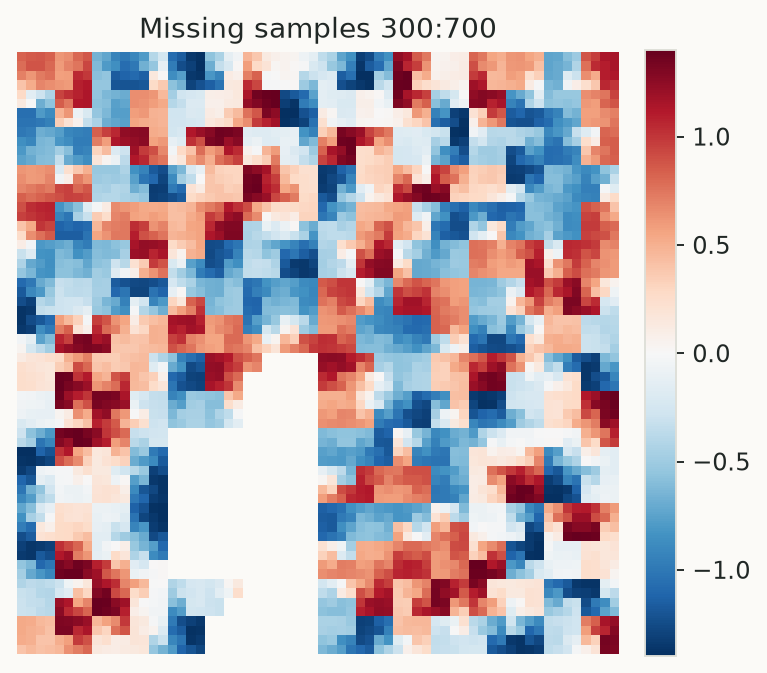
missing = values.copy()
missing[300:700] = np.nan
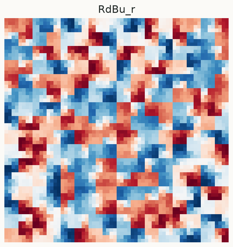
fig = hp.plot(missing, cmap="RdBu_r")

NaNs and masked samples are transparent in the data image. Infinities are rejected. Replace infinities using an explicit policy appropriate to the data before plotting.

Curve rendering

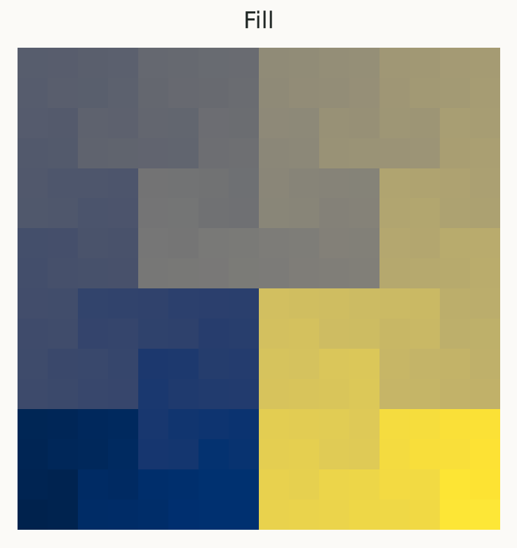
hp.plot_curve() displays a path, rather than measurement values. A solid color= uses one line color; cmap= colors visit order. mode="fill" colors cells by visit order. Automatic mode uses lines below order 8 and filled cells at larger orders.

Line mode shows the connected path.

Fill mode shows visit order as a field of colored cells.