Analysis examples
These examples use deterministic inputs and state what the transformation changes.
All figures are generated by
scripts/docs_gallery.py.
The Fourier and granularity datasets come directly from examples/readme_figures.py.
Thue–Morse: spatial spectral structure
Input: 1,048,576 binary terms, arranged on a 1024-square Hilbert grid.
Operation: mean subtraction, separable Hann window, centred 2-D FFT magnitude,
then log1p display scaling.
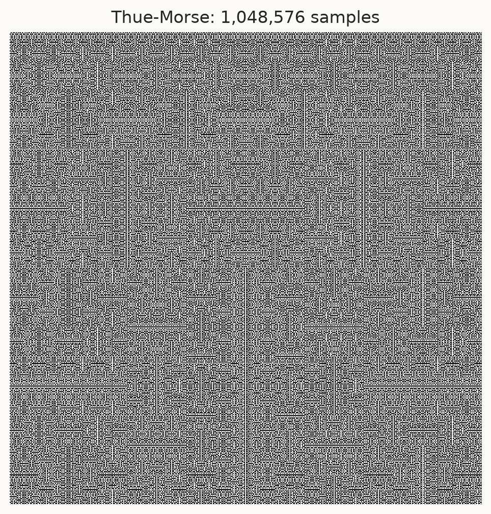
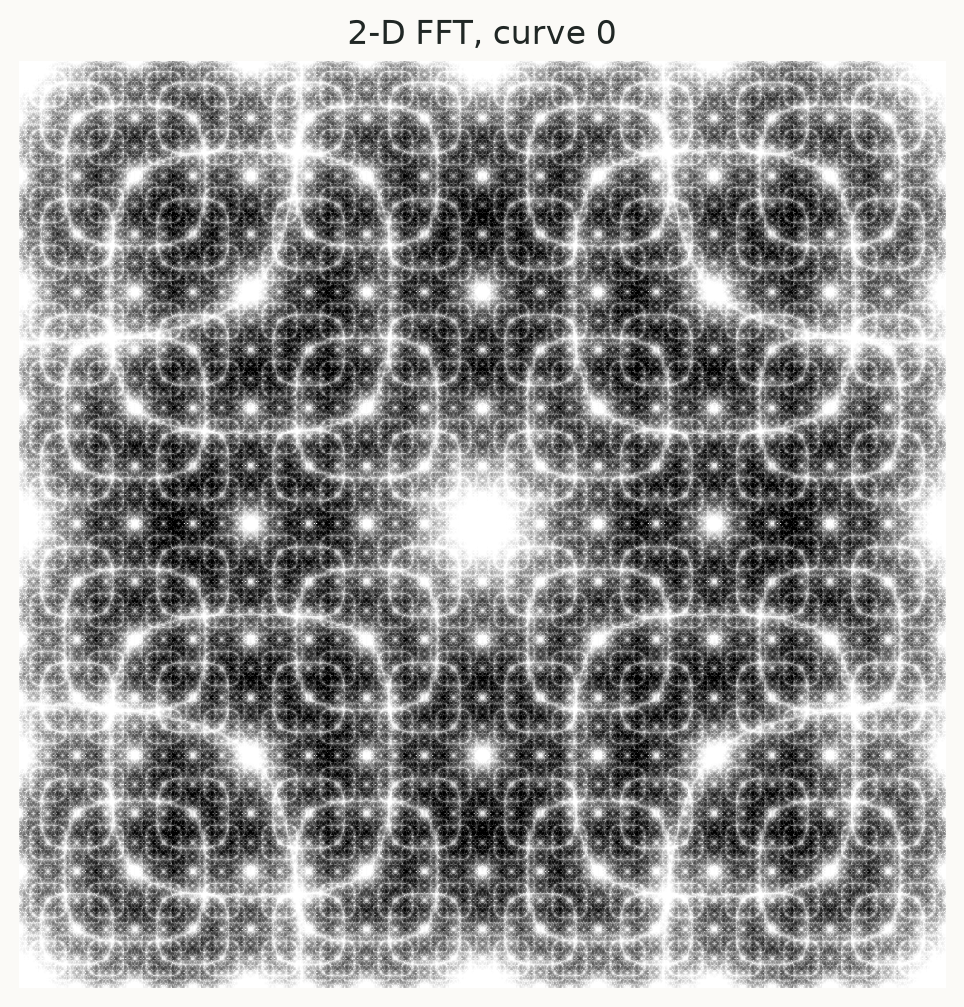
The spectral map displays repeated structure across scales. The input is aperiodic; its structure should not be described as a single hidden period. Changing the curve changes this spatial spectrum. Reproduction and interpretation.
Equal-density runs: separating periodic regions
Input: seeded interleaving of period-4 and period-6 binary runs with equal density. Operation: repeat the mean of each consecutive four-sample block.
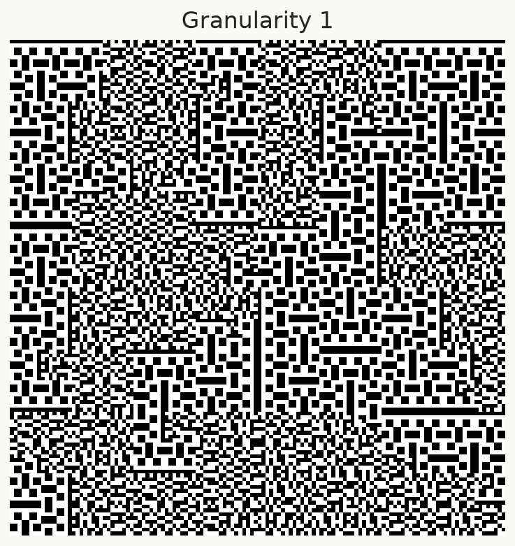
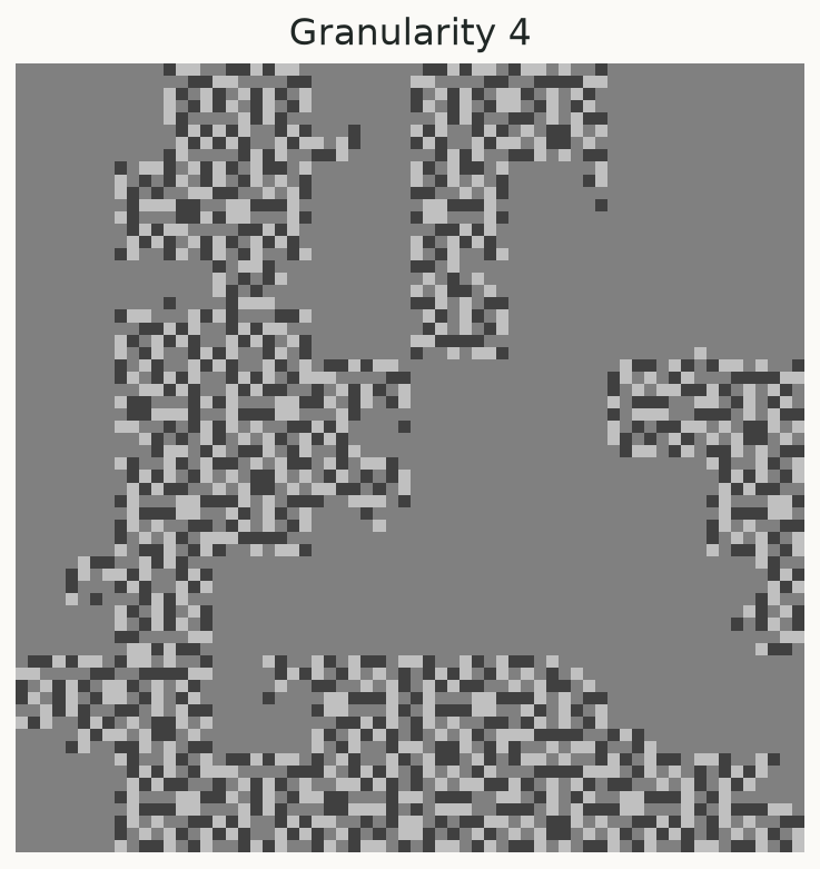
Period-4 runs become uniform while period-6 runs retain block variation. The regions are distinguished by response to averaging, not by different input means. Dataset construction and block-length dependence.
Curve locality: comparing geometric fields
Input: four curve constructions at the same resolution. Operation: average visit-index distance to up-to-eight spatial neighbours.
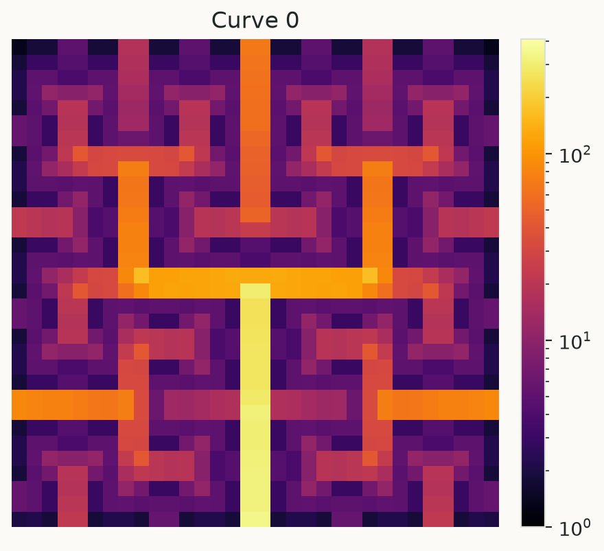
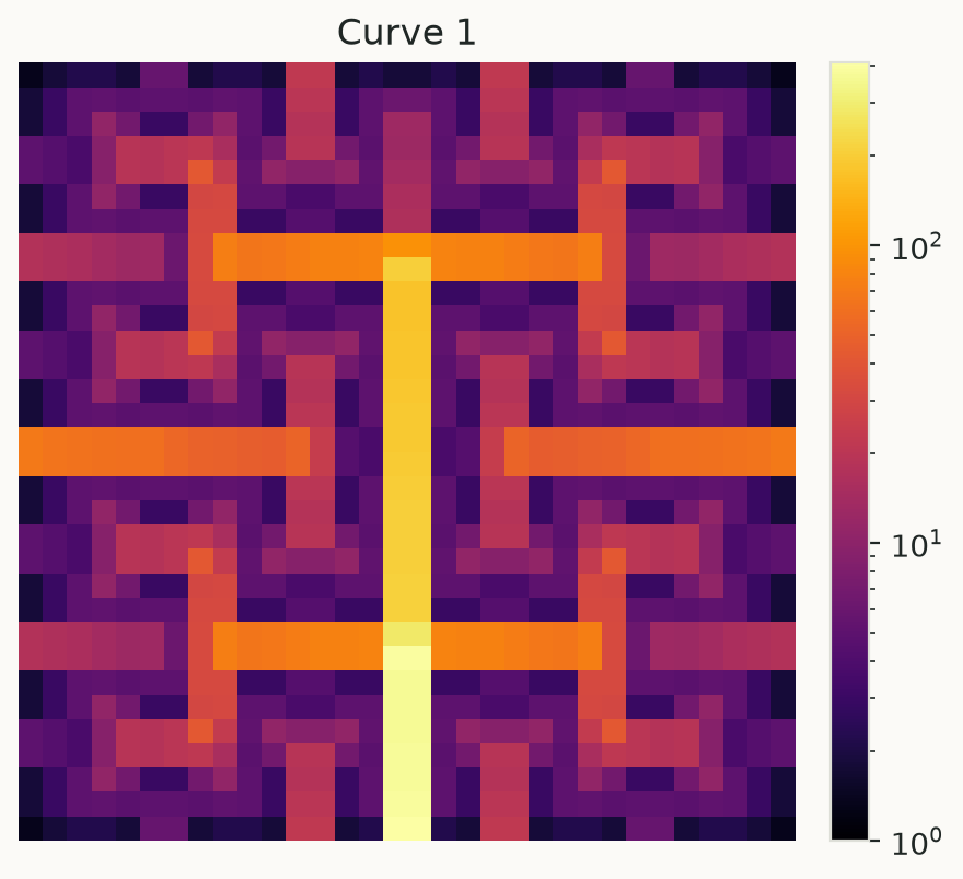
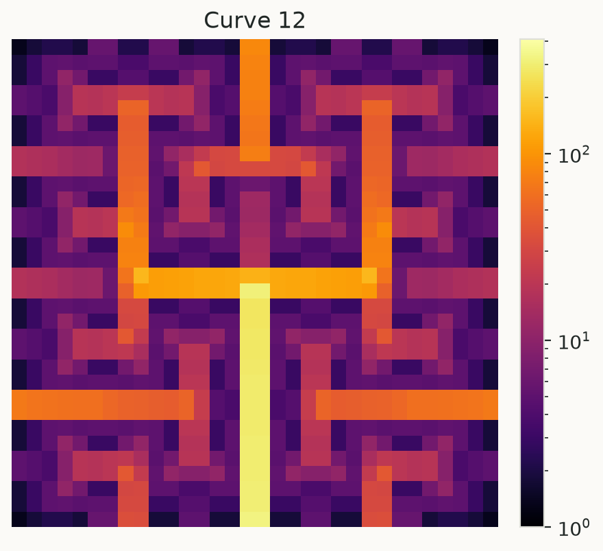
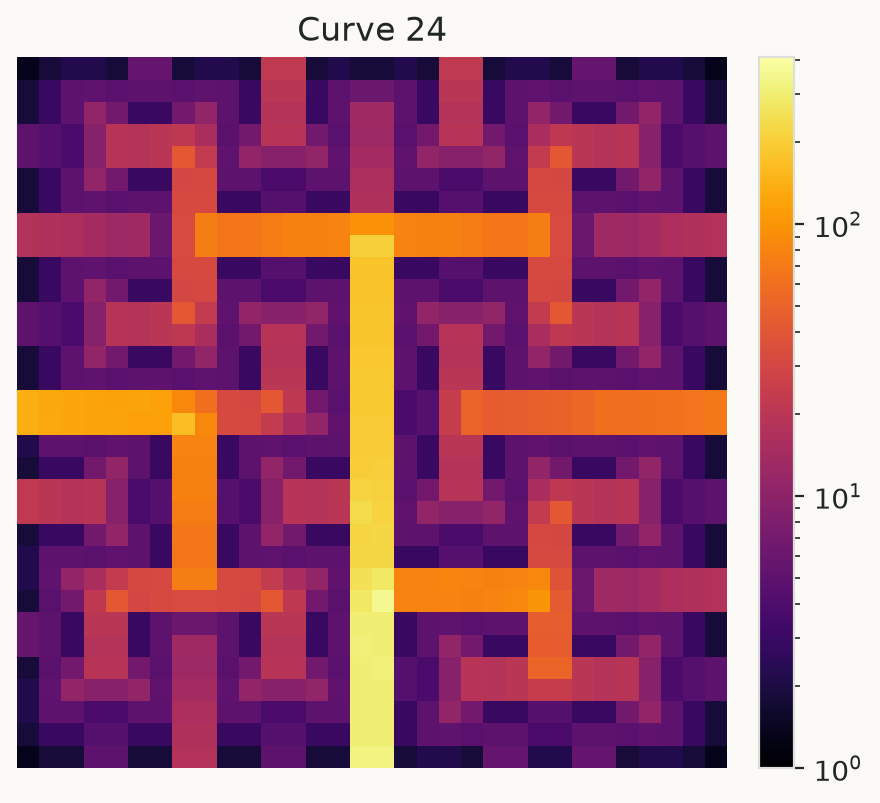
These plots do not use measurement values. The shared logarithmic scale makes both small and large distances visible. Field definition and numeric output.
RGB arrays: exact reconstruction and permutation
Input: a uint8 RGB test image containing a blue square, orange disk and green stripe. Operation: read its pixels along curve 0, then write the sequence using curve 0 or 12.
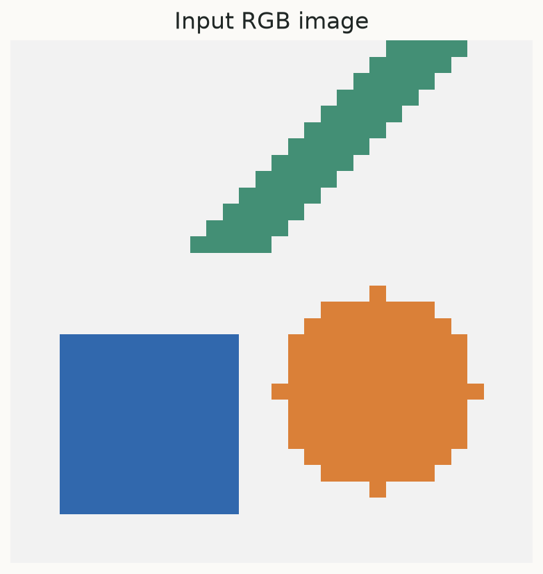
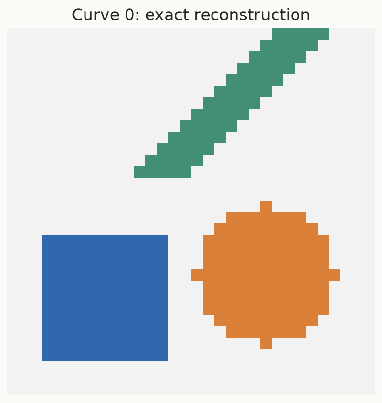
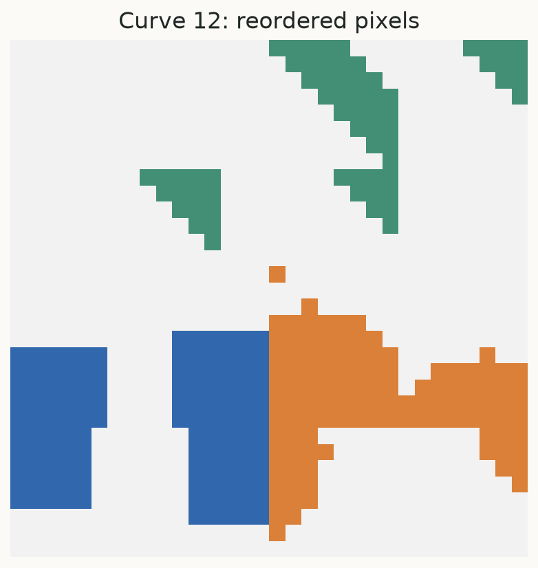
The same curve recovers every channel value exactly. A different curve changes spatial placement while retaining the pixels. Conversion guarantees.
Color normalization: positive values across several scales
Input: exp(3*sin(i/37)), ranging from approximately 0.05 to 20.09.
Operation: linear or logarithmic color normalization of the same mapped values.
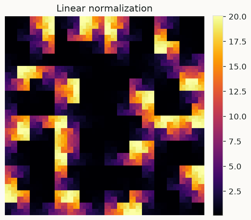
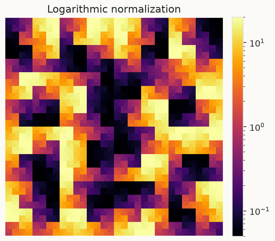
Logarithmic color normalization changes visibility across value ranges; it does not transform the stored array or calculate a Fourier spectrum. Plotting options.