Fourier maps

hp.plot(values, fourier=True) plots the centred 2-D FFT magnitude of the image obtained by mapping values along a curve. hp.data.fourier() returns the numeric spectrum. This is neither the original sequence’s 1-D FFT nor squared power.

Thue–Morse sequence

The binary Thue–Morse sequence starts at 0 and repeatedly appends its bitwise complement: 0 → 01 → 0110 → 01101001 → …. It is deterministic and aperiodic. This example uses \(4^{10}=1,048,576\) terms on a \(1024\times1024\) grid.

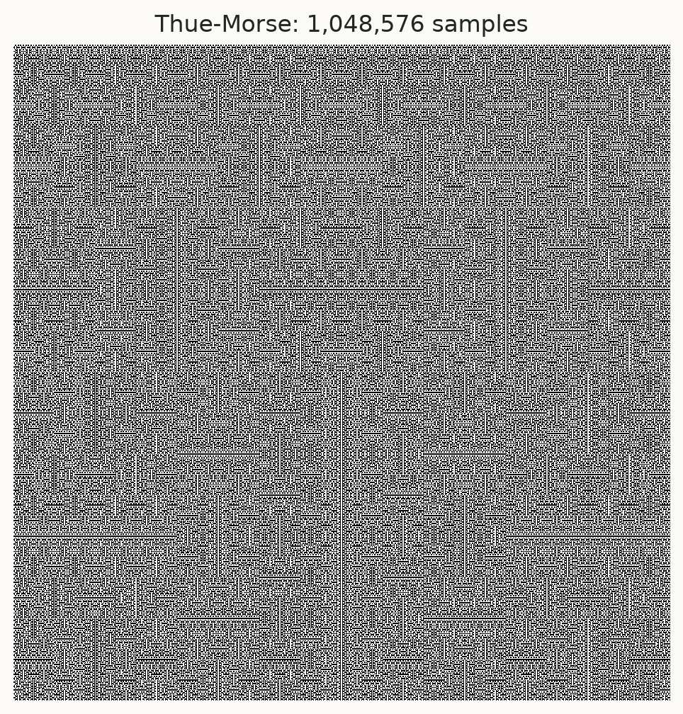
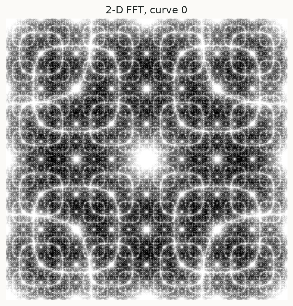
The direct image contains dense binary texture. Its Fourier map makes a repeated, multiscale spectral structure easier to identify. The mapping, mean subtraction, window and display contrast all affect the result; this image alone does not establish a fractal dimension or replace a quantitative spectral analysis.

Reproduce the figure

import numpy as np
import hilbertplot as hp

def thue_morse(n):
    sequence = np.array([0.0])
    while sequence.size < n:
        sequence = np.concatenate((sequence, 1 - sequence))
    return sequence[:n]

values = thue_morse(4**10)
fig = hp.plot(values, curve=0, cmap="gray", colorbar=False)
spectrum = hp.data.fourier(values, curve=0, window=True)
lo, hi = np.percentile(spectrum, [2, 99.5])
fig = hp.plot(values, curve=0, fourier=True, window=True,
              cmap="gray_r", vmin=lo, vmax=hi, colorbar=False)

The spectrum is displayed as log(1 + magnitude). In this reversed grayscale, darker pixels indicate larger values. The explicit 2nd and 99.5th percentile limits match the README example’s contrast policy. They affect colors only; the numeric spectrum is not clipped. The API’s automatic Fourier display limits are instead the 50th and 99.8th percentiles.

Exact transform pipeline

1. Apply optional granularity in sequence order, then map to the selected grid.

2. Replace missing cells with the mean of finite image values.

3. Subtract the image mean when remove_dc=True (the default).

4. Multiply by a separable Hann window when window=True (default False).

5. Compute abs(fftshift(fft2(image))).

6. Apply log1p when log=True (the default).

An image with no finite values raises an error. Complex input and infinity are rejected by the public plotting/Fourier interface. Raw array conversion can still preserve complex values.

Hann window

For a side of length \(N>1\), the weights are

\[w[k]=\tfrac12\left(1-\cos\frac{2\pi k}{N-1}\right).\]

With default mean subtraction, the image sent to the FFT is \(J[y,x]=(I[y,x]-\bar I)w[y]w[x]\). For five samples, the one-dimensional weights are [0, 0.5, 1, 0.5, 0]. Borders receive zero weight; the centre receives the largest weight.

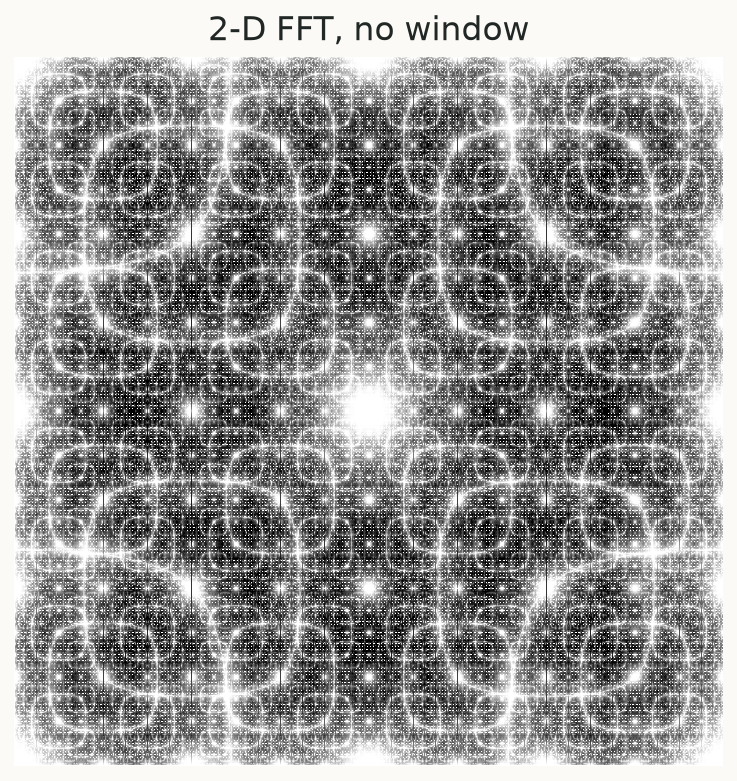
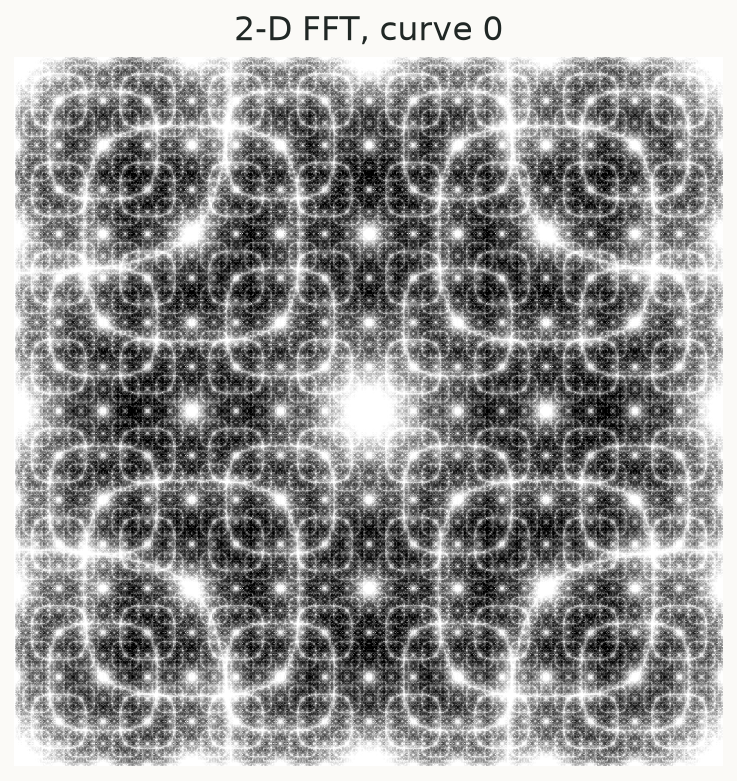
Tapering reduces discontinuities at the image edges, but changes amplitudes and broadens spectral peaks. There is no gain correction. NumPy’s length-one window is [1]; a length-two Hann window is all zeros.

Dependence on the curve

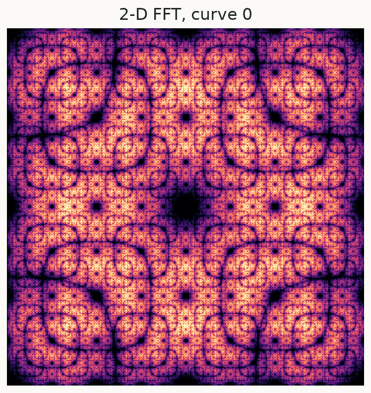
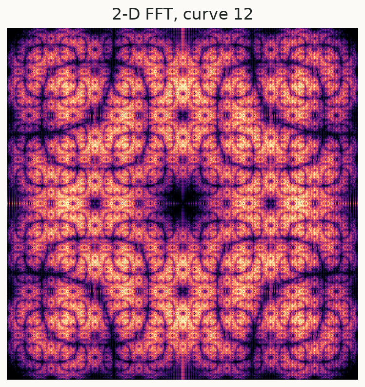
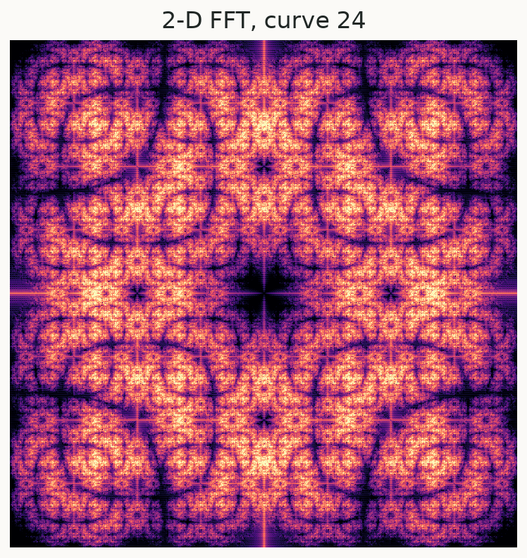
The same sequence produces different 2-D images under different curves and therefore different spectra. These three plots each use their own 2nd/99.5th percentile limits; compare their spatial structure, not absolute color amplitudes. Curve, grid size, padding, window, DC removal and scaling should be fixed for quantitative comparisons.

fourier=True and difference=True are mutually exclusive.