hilbertplot
Python library · 40 curve constructions
hilbertplot
Plot one-dimensional data along Hilbert curves. Read images as sequences, and reconstruct them along the same path or a different one.
pip install hilbertplotPython ≥ 3.10PyPIZenodo DOI
Start with your data
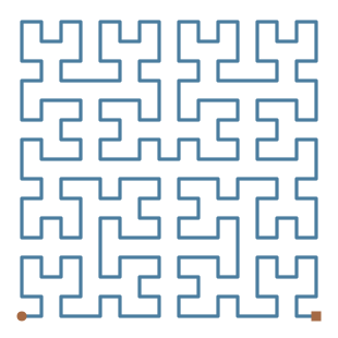
Choose a curve by its number, label or paper symbol. Plotting returns Matplotlib figures; conversion returns NumPy arrays.
Plot a sequence
Successive values fill successive cells along the selected curve.
import numpy as np
import hilbertplot as hp

values = np.sin(np.arange(4096) / 37)
fig = hp.plot(values, curve=0, cmap="cividis")
fig.savefig("sequence.png", dpi=180)
Read and reconstruct an image
Use the same curve and original shape for an exact round trip.
import numpy as np
import hilbertplot as hp

image = np.arange(256).reshape(16, 16)
sequence = hp.data.from_grid(image, curve=12)
restored = hp.data.to_grid(
    sequence, curve=12, shape=image.shape
)
np.testing.assert_array_equal(restored, image)
Analysis examples
A curve sets the arrangement. Fourier and granularity operations make different properties of that arrangement visible. Each example below links to its input, settings and mathematical definition.
01 / Fourier transform
The Thue–Morse sequence
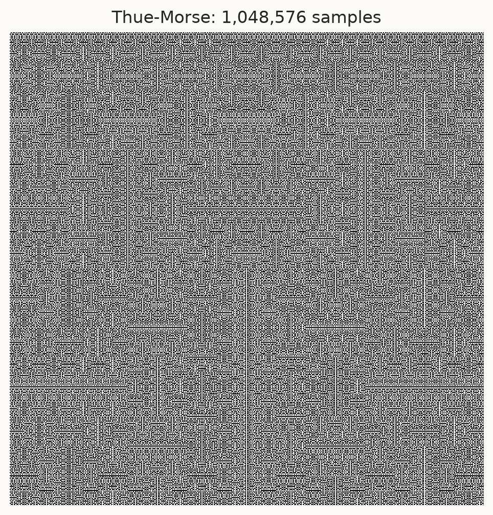
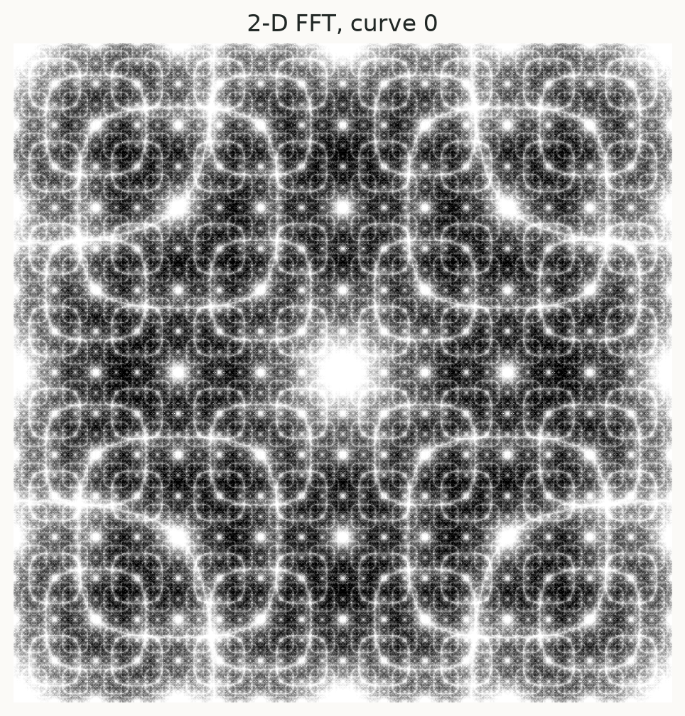
The same 1,048,576 binary values appear in both maps. The left map shows their placement along the Hilbert curve; the right shows the centred 2-D Fourier magnitude with a Hann window. Its multiscale spectral structure is easier to identify than in the direct image. This is the spectrum of the mapped image, not the sequence’s 1-D spectrum.
02 / Granularity
Distinguish periodic regions
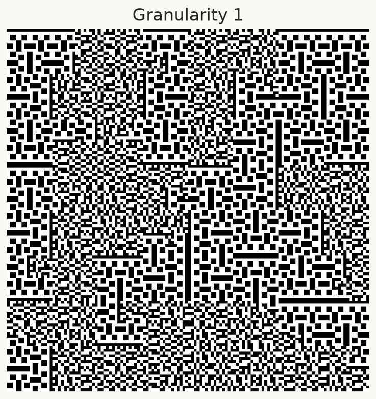
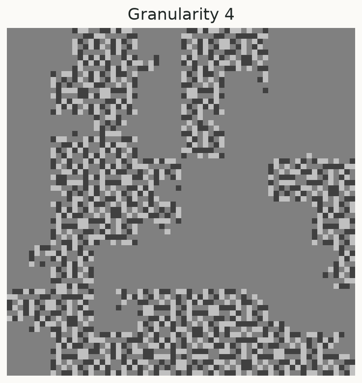
This sequence interleaves period-4 and period-6 runs, both with mean 1/2. Averaging consecutive blocks of four makes aligned period-4 runs uniform grey, while period-6 runs retain variation. The input length and curve stay the same.