How the curves are constructed

A curve in this library is an ordered path through grid cells. At order 1 it visits 4 cells; at order 2 it visits 16; at order 3 it visits 64. Each increase in order doubles both grid dimensions.

The classification describes how that path is assembled, not the measurements being plotted. Every construction covers the whole grid once. “Homogeneous” does not mean equal data values, and “improper” does not mean a broken path.

1. The building block: a lower-order path

To construct an order-3 path on an 8 × 8 grid, divide the grid into four 4 × 4 quadrants. Put an order-2 path in each quadrant, orient each copy appropriately, then connect the four paths.

The lower-order path put into a quadrant is called its kernel. A kernel is a whole ordered curve, not a single cell or a line segment. Two kernels used below are the standard Hilbert curve (index 0) and Liu4 (index 5):

Hilbert kernel: 16 visits. Entry (0,0), exit (3,0).

Liu4 kernel: 16 visits. Entry (0,1), exit (2,0).

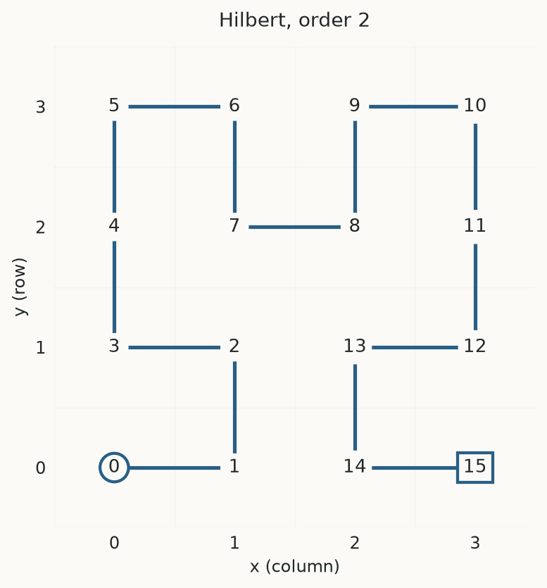
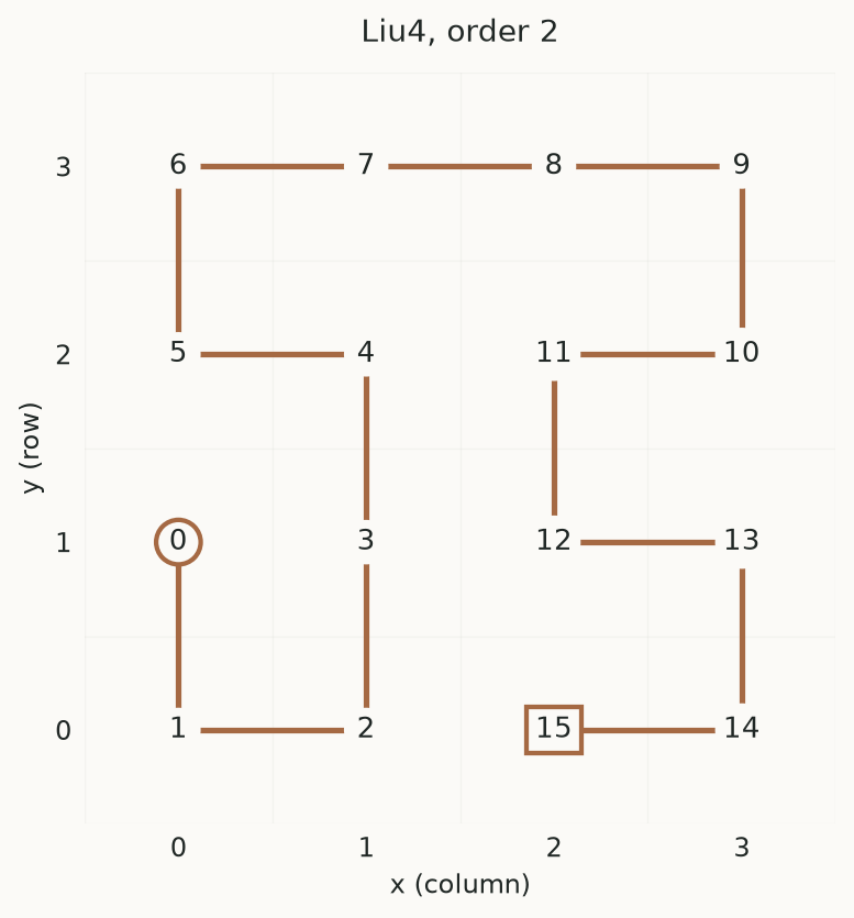
The numbers show visit order, not coordinates. The circle marks the first cell and the square the last. Hilbert enters and exits at adjacent corners of its square. Liu4 has a different path and its endpoints lie partway along two adjacent edges. Those endpoint positions matter when connecting quadrants.

2. Placement and traversal are separate operations

A kernel can be rotated or reflected to fit a quadrant. These operations move its cells. A reversal instead reads the same placed path backwards: its cells stay where they are, but its entry and exit exchange roles.

For a path P = [p0, p1, ..., p15], reversal is [p15, ..., p1, p0]. It changes which endpoint is reached first. It is not an image reflection.

The quadrants are visited in this order:

          +-----------------+-----------------+
          | Q1: second      | Q2: third       |
          |                 |                 |
          +-----------------+-----------------+
          | Q0: first       | Q3: fourth      |
          |                 |                 |
          +-----------------+-----------------+

                Q0 → Q1 → Q2 → Q3

A valid assembly requires the exit of each quadrant path to be one horizontal or vertical cell away from the entry of the next. Covering every cell is not sufficient if the path jumps across a gap.

3. Homogeneous: four copies of one kernel type

Consider Moore, curve 1, at order 3. All four quadrants contain the order-2 Hilbert kernel. The left two copies are rotated 90° counterclockwise; the right two are rotated 90° clockwise. The rotations differ, but the kernel type is the same in every quadrant. That makes the construction homogeneous.

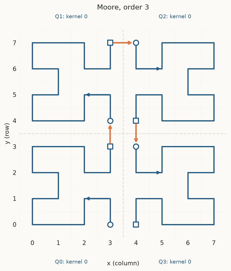
Here are the actual endpoints in the assembled 8 × 8 grid. Coordinates are (x,y), with the lower-left cell at (0,0).

Quadrant	Kernel	Placement	Entry	Exit
Q0, bottom left	Hilbert, order 2	90° counterclockwise	(3,0)	(3,3)
Q1, top left	Hilbert, order 2	90° counterclockwise	(3,4)	(3,7)
Q2, top right	Hilbert, order 2	90° clockwise	(4,7)	(4,4)
Q3, bottom right	Hilbert, order 2	90° clockwise	(4,3)	(4,0)

Read the table downwards: (3,3) → (3,4), then (3,7) → (4,7), then (4,4) → (4,3). Each connector is exactly one cell long.

“Four copies” does not mean four smaller Moore curves. For Moore at order 4, the quadrants contain Hilbert paths of order 3. The same distinction applies at higher orders: the selected construction specifies which kernel to use and how to place it.

4. Proper: the Hilbert-kernel homogeneous family

The proper constructions, indices 0–5, use the Hilbert kernel in all four quadrants, with the rotations/reflections specified by each construction. Hilbert, Moore and Liu1–Liu4 are different ways to assemble that same kernel.

Thus “proper” and “homogeneous” describe different aspects of Moore:

• It is homogeneous because all four quadrants use one kernel type.

• It is proper because that kernel is the standard Hilbert path and the assembly belongs to this rotation/reflection family.

Different placements give different global paths even though the constituent kernel is identical. Only curve 0 recursively uses its own Hilbert rule at every level; one must not repeatedly substitute the Moore rule into Moore quadrants.

5. Improper: the Liu4-kernel homogeneous family

The improper constructions, indices 6–11, start with four Liu4 kernels rather than four Hilbert kernels. Their assembly also uses reversal of selected quadrant paths. This produces six additional connected constructions.

The distinction is the kernel and its assembly rule; “improper” is not a claim that the resulting curve is invalid. The terminology and construction are from Pérez-Demydenko et al., sections 3–4.

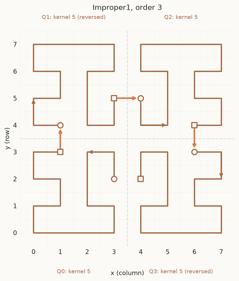
For Improper1, curve 6, at order 3:

Quadrant	Kernel	Placement and traversal	Entry	Exit
Q0	Liu4, order 2	Rotate 180°	(3,2)	(1,3)
Q1	Liu4, order 2	Reflect left/right, then reverse	(1,4)	(3,5)
Q2	Liu4, order 2	No rotation or reflection	(4,5)	(6,4)
Q3	Liu4, order 2	Reflect top/bottom, then reverse	(6,3)	(4,2)

Again, the connectors are unit steps: (1,3) → (1,4), (3,5) → (4,5), and (6,4) → (6,3).

Why reverse Q1? Reflecting its Liu4 path puts the endpoints at (3,5) and (1,4), in that traversal order. Q0 exits at (1,3), so entering Q1 at (3,5) would jump four grid edges. Reversing Q1 makes (1,4) its entry, which is just one step above Q0’s exit. The geometry within Q1 is unchanged; only traversal order changes. Q3 is reversed for the same connection requirement.

This remains homogeneous: every quadrant uses Liu4. Reversing a copy does not introduce a second kernel type.

6. Inhomogeneous: different kernel types within one assembly

Curve 12 uses Liu2 (index 3) in Q0 and Q3, and Liu4 (index 5) in Q1 and Q2. The quadrants therefore contain two different lower-order paths, not merely differently oriented copies of one path. It is inhomogeneous.

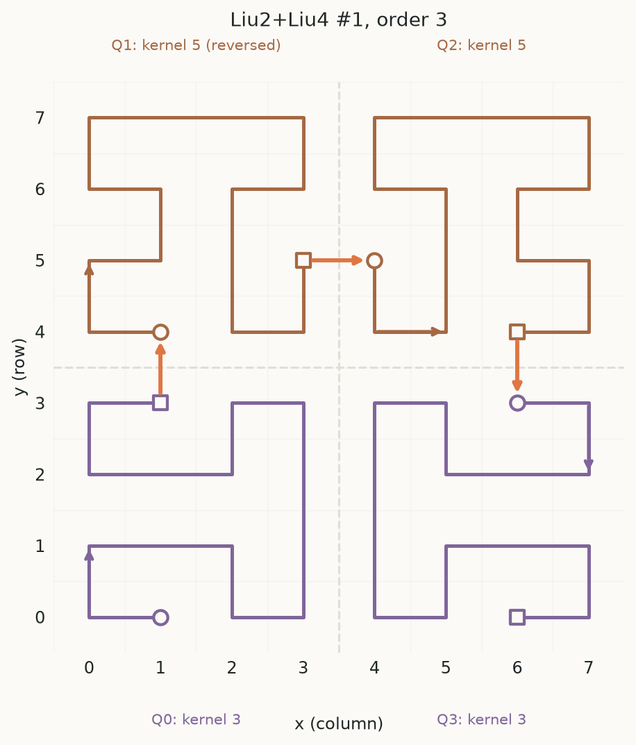
Quadrant	Kernel at order 2	Placement and traversal
Q0	Liu2	Reflect across the rising diagonal
Q1	Liu4	Reflect left/right, then reverse
Q2	Liu4	Unchanged
Q3	Liu2	Reflect across the falling diagonal

The component kernels can themselves be proper curves; that does not make the whole mixed construction a proper homogeneous curve. Classification concerns this assembly’s kernel choices.

Classification in the API

import numpy as np
import hilbertplot as hp

assert hp.curves.info("Moore")["kernels"] == [0]
assert hp.curves.info(6)["kernels"] == [5]
assert hp.curves.info(12)["kernels"] == [3, 5]

# Verify the three connections in the worked Moore example.
points = hp.curves.points("Moore", order=3)
quadrants = np.split(points, 4)
for previous, following in zip(quadrants[:-1], quadrants[1:]):
    assert np.abs(previous[-1] - following[0]).sum() == 1

Group	What is held the same?	Indices	API selection
Proper homogeneous	Hilbert kernel in every quadrant	0–5	hp.curves.proper()
Improper homogeneous	Liu4 kernel in every quadrant, with reversal in the rules	6–11	hp.curves.improper()
All homogeneous	One kernel type per construction	0–11	hp.curves.homogeneous()
Inhomogeneous	At least two kernel types in one construction	12–39	hp.curves.inhomogeneous()

hp.curves.by_kernels(3, 5) selects an exact set of kernel types, not any curve containing either kernel. Metadata’s rule records placements and reversals; kernels records only the distinct kernel indices.

Other properties: closed paths and supported shapes

A closed construction has entry and exit that can be joined to form a loop. For example, the Moore path above starts at (3,0) and ends at (4,0), so a single final edge joins them. The plotting function draws the finite ordered path; it does not add a new data sample for that closing edge.

Generalizing means that the library can construct connected paths on arbitrary squares and quasisquares, beyond power-of-two side lengths. This is a separate property, not another name for homogeneous. A quasisquare has sides differing by one; general rectangles are unsupported.

assert [c["index"] for c in hp.curves.generalizing()] == [0, 3, 4, 5, 24, 29, 30, 31]
fig = hp.plot_curve(3, shape=(15, 16), color="steelblue")

All forty curves work on power-of-two squares. The catalog shows their paths; fitting explains how data length selects a grid.