Convert arrays along a curve

The conversion functions rearrange numeric values. They preserve dtype and masks without normalization. With no averaging or truncation, a round trip recovers the input exactly.

Sequence → grid → sequence

import numpy as np
import hilbertplot as hp

values = np.arange(100, dtype=np.uint64) + 2**63
grid = hp.data.to_grid(values, curve=12)
recovered = hp.data.from_grid(grid, curve=12, length=len(values))
np.testing.assert_array_equal(recovered, values)
assert recovered.dtype == values.dtype

to_grid() puts successive values into successive curve cells. from_grid() visits those cells in the selected curve’s order and reads their contents.

For four values on the standard Hilbert curve:

Sequence: [10, 20, 30, 40]
Grid array, row 0 first:
[[10, 40],
 [20, 30]]

Reading this array normally by rows gives [10, 40, 20, 30]. Reading along the same curve with from_grid() gives [10, 20, 30, 40].

Image → sequence → image

image = np.arange(16 * 16, dtype=np.uint16).reshape(16, 16)
sequence = hp.data.from_grid(image, curve=12)
restored = hp.data.to_grid(sequence, curve=12, shape=image.shape)
np.testing.assert_array_equal(restored, image)

Keep the original shape when reconstructing. Without shape=, the default fitting policy chooses a new grid based on sequence length.

Colour images

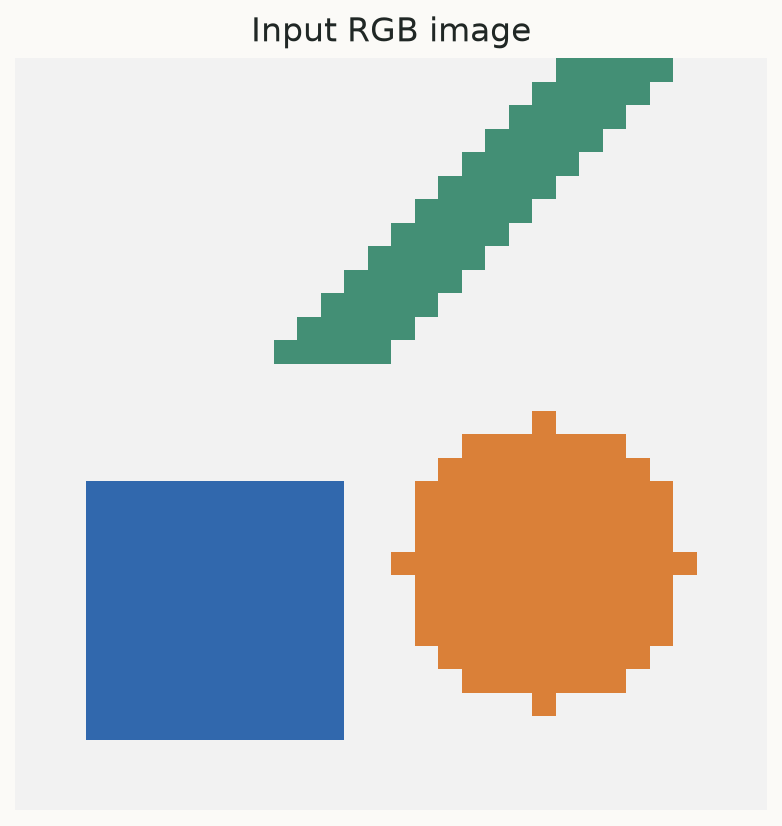
y, x = np.mgrid[0:32, 0:32]
rgb = np.full((32, 32, 3), 242, dtype=np.uint8)
rgb[3:14, 3:14] = [49, 104, 173]                         # blue square
rgb[(x - 22)**2 + (y - 10)**2 <= 36] = [218, 128, 56]  # orange disk
rgb[(y > 18) & (np.abs(x - y + 6) < 3)] = [67, 143, 117] # green stripe
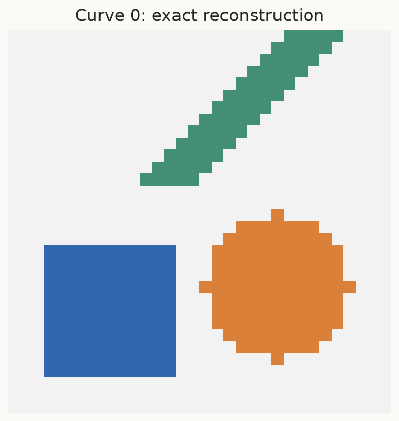
sequence = hp.data.from_grid(rgb, curve=0)
assert sequence.ndim == 1
assert sequence.size == rgb.size
restored = hp.data.to_grid(sequence, curve=0, shape=rgb.shape)
np.testing.assert_array_equal(restored, rgb)
assert restored.dtype == np.uint8

Each pixel’s channels stay consecutive and in their original order. The spatial path selects pixels; channels are then read within each pixel. Pass the full original shape, including channel dimensions, when reconstructing a flat colour sequence. RGBA and additional trailing component axes follow the same convention.

length= counts flattened values, including channels. Omit it when reading a complete image.

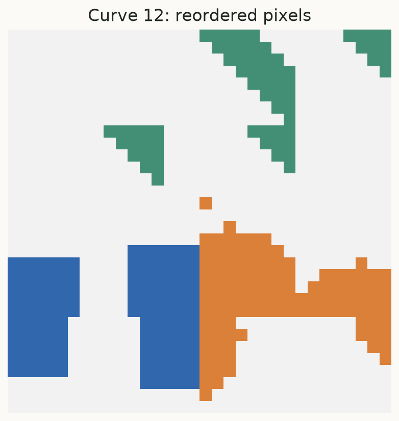
The figure below uses this exact uint8 image. The first reconstruction uses the same curve; the final image writes the sequence with curve 12 instead. That changes pixel placement, as described under reordering.

Supported image shapes

Power-of-two squares work with all forty curves. Arbitrary squares and quasisquares work with curves 0, 3, 4, 5, 24, 29, 30, 31. General rectangles are unsupported and raise an error. No pixels are silently cropped, skipped, or assigned a different curve.

Reorder with a different curve

values = np.arange(64)
grid = hp.data.to_grid(values, curve=0)
reordered = hp.data.from_grid(grid, curve=12)

# Reverse the reordering using the same grid size.
restored_grid = hp.data.to_grid(reordered, curve=12)
original = hp.data.from_grid(restored_grid, curve=0)
np.testing.assert_array_equal(original, values)

A different curve creates a permutation. Keep every grid entry, including padding, while reversing that permutation; reading with another curve can move padding into the middle.

Complex values and infinities are allowed in raw conversion. Plotting and Fourier-map rendering require real scalar sequences with finite values or NaNs for missing entries.