Locality and difference maps

Consecutive samples follow adjacent grid cells. Spatial neighbours can nevertheless have widely separated sequence indices. A difference map measures that separation; it is a property of the curve and resolution, independent of measurement amplitudes.

Let \(L[y,x]\) be the visit index of cell \((x,y)\), and let \(\mathcal N(x,y)\) contain its in-bounds horizontal, vertical and diagonal neighbours. The map is

\[D[y,x] = \frac{1}{|\mathcal N(x,y)|} \sum_{(u,v)\in\mathcal N(x,y)} |L[y,x]-L[v,u]|.\]

Interior cells have eight neighbours, non-corner edge cells five, and corners three. A single-cell grid returns zero.

Comparing curves

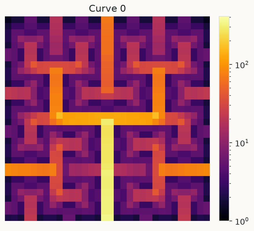
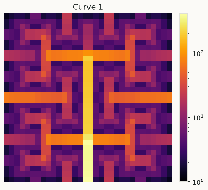
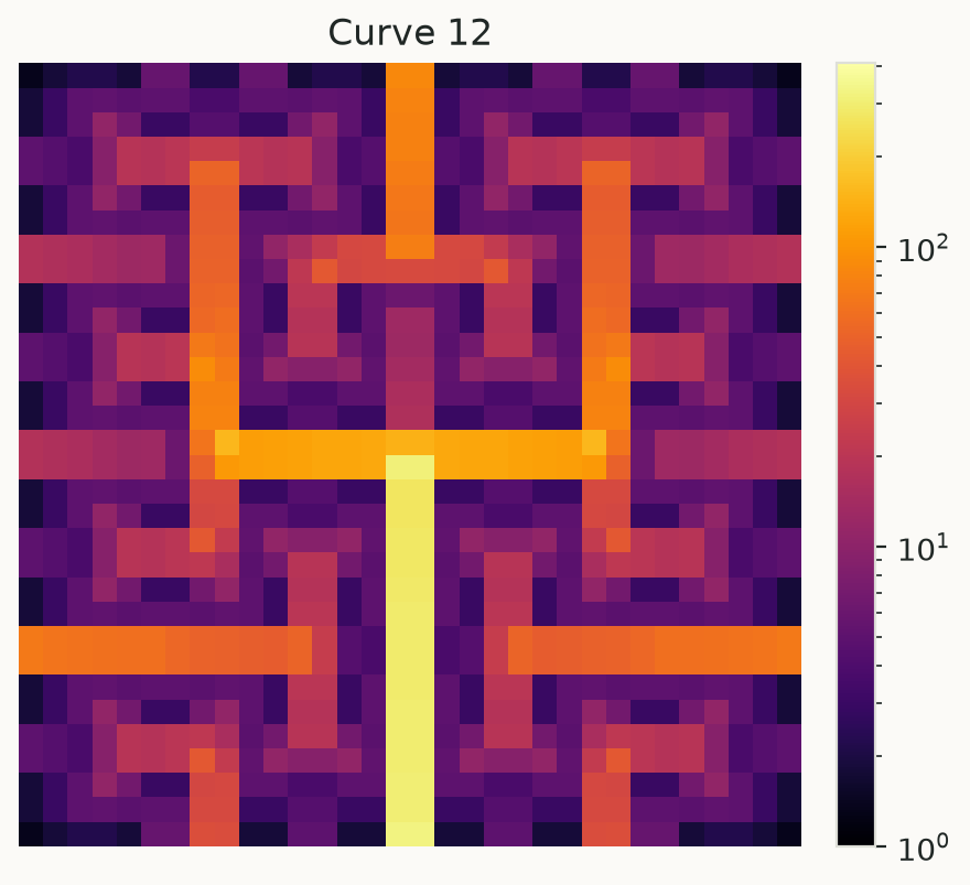
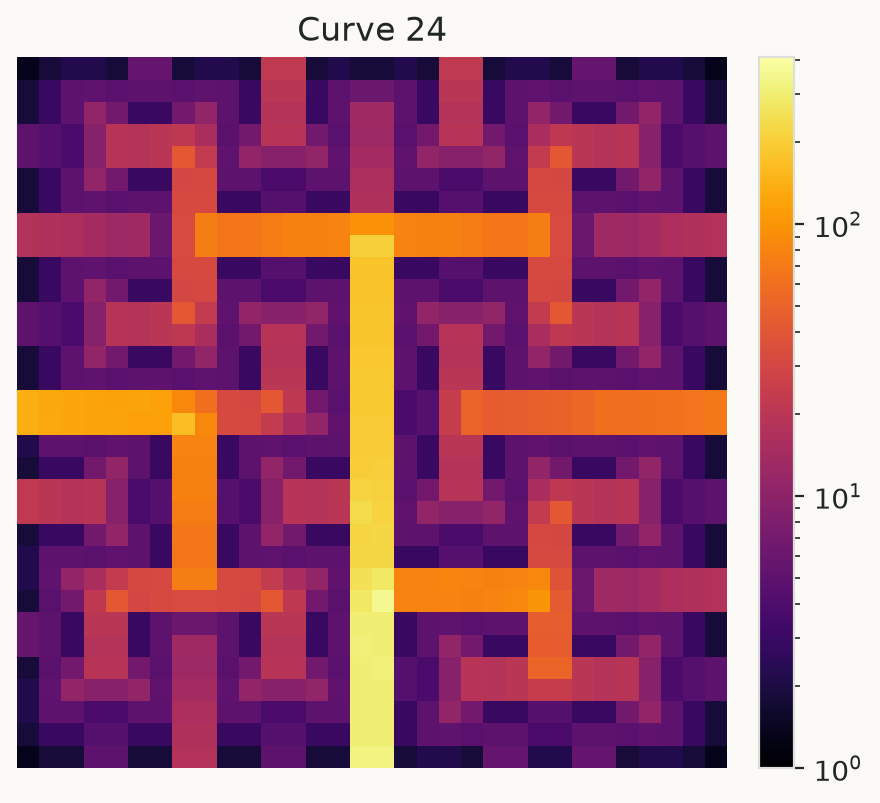
These maps use the same 32-square resolution, inferno colormap and logarithmic normalization. Low distances remain visible while large jumps at region boundaries can still be compared. Colorbar values are mean visit-index distances; logarithmic normalization changes display, not the computed field.

import numpy as np
import hilbertplot as hp
from matplotlib.colors import LogNorm

values = np.arange(4**5)
field = hp.curves.difference_map(0, order=5)
fig = hp.plot(values, curve=0, difference=True, cmap="inferno",
              norm=LogNorm(vmin=1, vmax=field.max()))

A consistent comparison should use a shared vmax, such as the maximum across all fields being compared. Do not use logarithmic normalization for a one-cell zero field.

Matching a data plot’s grid

values = np.arange(900)
grid = hp.data.to_grid(values, curve=0, fit="square")
field = hp.curves.difference_map(0, side=grid.shape[0])
labels = hp.curves.label_map(0, side=grid.shape[0])
assert field.shape == grid.shape == labels.shape

hp.plot(values, difference=True) uses its fitted grid size; numerical difference_map() takes a power-of-two order or an explicit square side. Granularity changes values, not this geometric field. Fourier and difference flags cannot be enabled together. The difference map fills the complete image.