Work · Tune

Tune

Eight parameters account for most of the variance in forecast quality. Tune them by hand first, since each has a direction you can reason about, then use run_hpo to search over their interactions.

Parameter	Controls	Range	First move
reservoir_size	model capacity	100–2000	double it until gains stall
spectral_radius	memory horizon, stability	0.8–1.2	sweep ±0.1 around 0.9
leak_rate	state update timescale	0.05–1.0	lower it for slow signals
bias_scaling	diversity of unit operating points	0.0–2.0	leave at 1.0; 0.0 recovers pre-0.5 dynamics
topology	recurrent connectivity structure	registry names	default (dense random) first, graphs after
feedback_initializer	how the signal enters	registry names	default first; scale before structure
alpha	readout ridge regularization	1e-8–1e-2	step by ×100 on a log scale
warmup length	state synchronization	100–500 steps	raise it until forecasts stop changing

Spectral radius scales the recurrent matrix so its largest eigenvalue magnitude hits the target, which sets how long an input echoes through the state. Small values forget fast and stay stable; values near one remember longer and produce richer transients at the edge of instability — for driven, leaky reservoirs the best value often sits slightly above 1.0. This is the single most effective parameter for forecast horizon. Factories default to 0.9; a bare ESNLayer leaves the matrix unscaled unless you pass a value.

Leak rate blends the previous state into the new one: \(x_t = (1-a)\,x_{t-1} + a\,\tilde{x}_t\). At 1.0 the state is fully replaced each step (the standard ESN); smaller values integrate slowly, matching the reservoir's timescale to the signal's. Slow, smooth signals call for small leak rates; leak_rate=0.1 with a spectral radius near 1.0 is a standard configuration for long-period oscillations.

Alpha sets the bias–variance tradeoff of a ridge readout such as CGReadoutLayer. Too small, and the readout amplifies state noise and forecasts diverge within a few steps; too large, and predictions over-smooth toward the mean. The optimum shifts with reservoir size and training length, which is why it belongs in every search space.

---

Searching with run_hpo

Three callables define a study: a model factory, a search space, and a data loader. Each trial builds a fresh model, fits the readout, forecasts over the validation window, and scores it.

import resdag as rd
from resdag.hpo import run_hpo

data = ...                                  # (1, 2300, 3) — (batch, time, features)
warmup, train, target, f_warmup, val = rd.utils.prepare_esn_data(
    data, warmup_steps=200, train_steps=1600, val_steps=300
)

def model_creator(reservoir_size, spectral_radius, leak_rate, alpha):
    """One fresh model per trial. Must accept every key of search_space."""
    return rd.classic_esn(
        reservoir_size=reservoir_size, feedback_size=3, output_size=3,
        spectral_radius=spectral_radius, leak_rate=leak_rate,
        readout_alpha=alpha,
    )

def search_space(trial):
    return {
        "reservoir_size": trial.suggest_int("reservoir_size", 100, 500, step=100),
        "spectral_radius": trial.suggest_float("spectral_radius", 0.5, 1.2),
        "leak_rate": trial.suggest_float("leak_rate", 0.2, 1.0),
        "alpha": trial.suggest_float("alpha", 1e-8, 1e-2, log=True),
    }

def data_loader(trial):
    """Must return exactly these five keys, each (batch, time, features)."""
    return {"warmup": warmup, "train": train, "target": target,
            "f_warmup": f_warmup, "val": val}

study = run_hpo(
    model_creator=model_creator,
    search_space=search_space,
    data_loader=data_loader,
    n_trials=100,
    loss="efh",
    seed=42,
    storage="study.log",                    # journal file: resumable
)
print(study.best_params)

The data contract is validated per trial: the dict must contain "warmup", "train", "target", "f_warmup", "val", all 3-D tensors. The forecast horizon defaults to val.shape[1]. Input-driven models add drivers_keys=["driver"] and supply warmup_driver, train_driver, f_warmup_driver, and forecast_driver entries — the last one sliced with the pinned alignment.

Silent failures by design

catch_exceptions=True (the default) converts any per-trial error into penalty_value (1e10) and stashes the message in the trial's "error" attribute, so a single bad configuration cannot abort a long-running study. If most trials report 1e10, the exceptions are going unread — pass catch_exceptions=False while debugging.

Losses

Key	Behavior
"efh"	Expected forecast horizon — soft survival sum (default, chaotic systems)
"forecast_horizon"	Hard count of contiguous below-threshold steps
"lyapunov"	Error weighted by \(e^{-t/\tau}\) with lyapunov_t
"standard"	Mean geometric-mean error — stable or periodic signals
"soft_horizon"	Hill-gated survival horizon — smoother search landscape

All are minimized; the horizon losses are negated internally, so lower study values mean longer usable forecasts. loss_params passes kwargs (thresholds, metrics) to the chosen loss; monitor_losses=["standard"] logs extra metrics on every trial without optimizing on them.

Multi-worker studies

study = run_hpo(..., n_trials=200, n_workers=8, storage="study.log", seed=42)

Workers are separate OS processes coordinating through the storage file. Journal storage ("study.log") is append-only and handles concurrent writers; a .db path uses SQLite with WAL mode. BLAS threads are throttled to one per worker before forking, and re-running with the same storage and study name resumes where the study stopped.

Seed semantics differ by mode. Single-worker runs are fully reproducible: seed seeds the sampler, and each trial reseeds torch/numpy with seed + trial.number. Multi-worker runs derive a sampler seed per worker (seed + i·7919), but trial numbers are claimed in arrival order — so per-trial seeds, and hence the exact trial sequence, vary run to run even with a fixed seed.

---

Reading a study

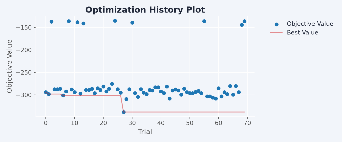
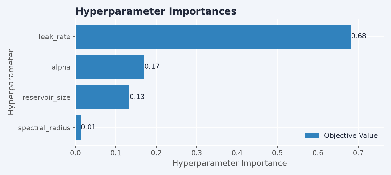
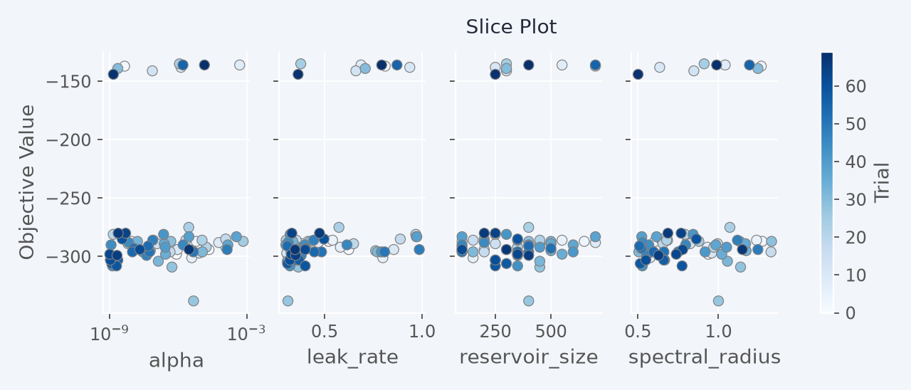
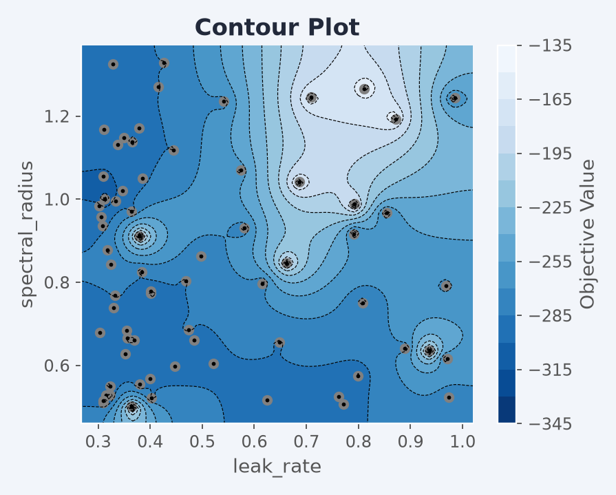
run_hpo returns a plain optuna study, so optuna's visualization module works on it directly: optuna.visualization for interactive plotly figures, optuna.visualization.matplotlib for static ones like the four below, drawn from a 70-trial study maximizing valid horizon on Lorenz.

from optuna.visualization import plot_optimization_history   # plotly, interactive
from optuna.visualization.matplotlib import plot_contour     # static

plot_optimization_history(study)

Per-trial objective with the running best.

Relative importance of each hyperparameter for the objective.

Slice plots: the objective against each parameter individually.

The spectral-radius × leak-rate landscape around the optimum.

Next

• Scale & deploy — run the best configuration at scale
• Reference · HPO — every run_hpo parameter