Build

Composing models¶

ResDAG treats reservoir architectures as directed acyclic graphs: reservoirs, augmentations, concatenations, and readouts, composed in whatever order the problem requires. Instead of monolithic model classes, the library provides individual layers and a functional API. You declare symbolic inputs, call layers on them, and wrap the resulting graph in ESNModel. Every page in this section builds on that pattern.

Composition patterns¶

The five patterns below cover the most common architectures in the reservoir computing literature. All use the same imports and run as written:

from resdag import (
    CGReadoutLayer, Concatenate, ESNLayer, ESNModel,
    SelectiveExponentiation, reservoir_input,
)

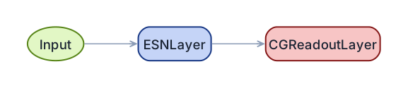
Minimal ESN — the base architecture that the other patterns extend.

inp = reservoir_input(3)
states = ESNLayer(200, feedback_size=3)(inp)
out = CGReadoutLayer(200, 3, name="output")(states)
model = ESNModel(inp, out)          # (batch, time, 3) -> (batch, time, 3)

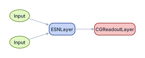
Minimal ESN architecture — One reservoir, one readout.

Input-driven — the first input is always the feedback signal; further inputs are exogenous drivers.

feedback = reservoir_input(1)
driver = reservoir_input(5)
states = ESNLayer(150, feedback_size=1, input_size=5)(feedback, driver)
out = CGReadoutLayer(150, 1, name="output")(states)
model = ESNModel([feedback, driver], out)

Input-driven architecture — Feedback plus a known exogenous series.

State augmentation, Ott-style — square the even-indexed states and let the readout see the raw input; this is what the ott_esn factory builds.

inp = reservoir_input(3)
states = ESNLayer(500, feedback_size=3)(inp)
augmented = SelectiveExponentiation(index=0, exponent=2.0)(states)
features = Concatenate()(inp, augmented)
out = CGReadoutLayer(3 + 500, 3, name="output")(features)
model = ESNModel(inp, out)

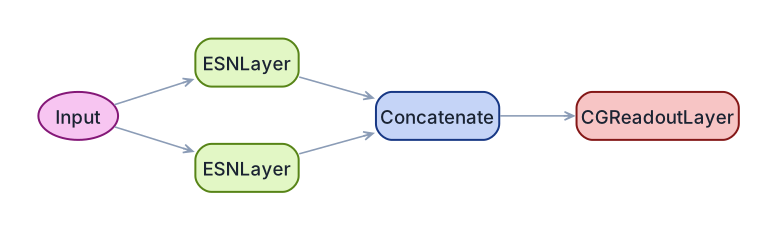
Ott ESN architecture — The `ott_esn` architecture, built layer by layer.

Parallel two-timescale reservoirs — a fast and a slow reservoir read the same signal; the readout mixes their features.

inp = reservoir_input(3)
fast = ESNLayer(120, feedback_size=3, leak_rate=1.0, spectral_radius=0.7)(inp)
slow = ESNLayer(120, feedback_size=3, leak_rate=0.2, spectral_radius=0.95)(inp)
merged = Concatenate()(fast, slow)
out = CGReadoutLayer(240, 3, name="output")(merged)
model = ESNModel(inp, out)

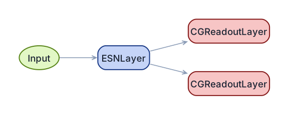
Parallel reservoirs architecture — Two timescales, one readout.

Multi-readout — one reservoir, two named heads, fitted together in a single ESNTrainer.fit call keyed by name.

inp = reservoir_input(3)
states = ESNLayer(300, feedback_size=3)(inp)
coords = CGReadoutLayer(300, 3, name="coords")(states)
energy = CGReadoutLayer(300, 1, name="energy")(states)
model = ESNModel(inp, outputs=[coords, energy])

Multi-readout architecture — Readout names become the keys of the targets dict.

In this section¶

Layers

Reservoir layers such as ESNLayer and NGReservoir, their parameters, and the transform layers used to connect them.
Readouts

Output layers fitted algebraically rather than by gradient descent. Currently CGReadoutLayer, a ridge regression readout solved by conjugate gradient.
Architectures

The premade model factories, the graph each one builds, and patterns for hand-built DAGs: stacked reservoirs, driving inputs, multiple readouts.
Initialization

Weight initialization for reservoirs: graph topologies, input and feedback initializers, plain callables, torch.nn.init functions, and the registry system that resolves names. Includes a catalog of every registered topology and initializer.