Work · Forecast

Forecast

forecast() runs two phases: a teacher-forced warmup that synchronizes the reservoir on real data, then horizon steps in which each output becomes the next feedback input. The rest of this page covers the indexing and alignment around that loop, which is where most forecast errors originate.

Anatomy

preds = model.forecast(f_warmup, horizon=2000)     # (batch, 2000, features)

Phase 1 resets the reservoirs (pass reset=False to continue from a saved state instead), runs a teacher-forced pass over f_warmup, and keeps the outputs. Phase 2 then makes horizon genuinely autoregressive model calls, each feeding the previous output back in. Prediction 0 is a real forecast step — the model's own output seeded by the last warmup output (or initial_feedback), not an echo of it — so horizon=1 returns one genuine forecast and return_warmup=True adds no duplicated frame at the warmup/forecast seam. The returned tensor aligns one-to-one with the val split from prepare_esn_data, so error metrics can be computed element-wise with no further index arithmetic.

Two optional arguments:

full = model.forecast(f_warmup, horizon=2000, return_warmup=True)
# (batch, warmup_steps + 2000, features) — teacher-forced outputs prepended;
# useful for plotting the handover from teacher forcing to autoregression

preds = model.forecast(f_warmup, horizon=2000, initial_feedback=seed)
# seed: (batch, 1, feedback_dim) — replaces the last warmup output as the
# first autoregressive input

Multi-output models return a tuple with the same structure. The first output is the one fed back, so its dimension must equal the feedback input's — a mismatch raises immediately, listing the model's readouts. The remaining outputs are computed at each step but do not enter the loop.

---

Driver alignment

Training pairs (feedback_t, driver_t) → feedback_{t+1}. The forecast loop keeps that pairing, which pins where the forecast drivers must start and how many steps you need:

warmup window    [0 .......... T)      feedback and drivers, teacher-forced
forecast window  [T ... T + horizon)   feedback generated by the model,
                                       drivers supplied by you

Forecast drivers start at T — the first step after the warmup window, exactly where the warmup drivers ended — and horizon steps are consumed, one per autoregressive step: the loop is fully autoregressive, so step t of the forecast window pairs the model's own feedback with forecast_inputs[:, t]. Slicing both windows from one full driver series d:

T, horizon = 200, 300

preds = model.forecast(
    (x[:, :T], d[:, :T]),                      # warmup: feedback + driver
    forecast_inputs=(d[:, T : T + horizon],),  # drivers continue at T
    horizon=horizon,
)
truth = x[:, T : T + horizon]                  # preds align with this

The driver window matches your validation targets exactly: both span [T, T + horizon). Supplying more than horizon steps is accepted — only the first horizon are consumed — but fewer raises. The validator is strict because misaligned drivers fail silently: shifted by one step, the model trains without error and only the forecast quality degrades. Theory · Timing derives the alignment index by index.

---

Windowed reconstruction

windowed_forecast() fills the gaps in a sparsely-observed trajectory. You hold the full ground-truth series but only trust it in periodic windows; between them the model free-runs. Each cycle re-synchronizes the reservoir on a short teacher-forced window, then forecasts across the unobserved gap — and because the Echo State Property re-anchors the state on every observed window, per-window error does not compound across windows, so gaps can be filled indefinitely. It is a thin @torch.no_grad() loop over forecast(): the reservoir is reset once (on the first window, and only when reset=True) and its state is carried across the whole pass.

[== warmup W ==][~~ gap P ~~][= teacher F =][~~ gap P ~~][= F =] ...
   observed        filled        observed       filled       obs
 (teacher-forced) (forecast)  (teacher-forced) (forecast)

recon, mask = model.windowed_forecast(
    series,            # (batch, T, feedback_dim) ground truth
    predict_len=200,   # P: autonomous steps per gap
    teacher_len=40,    # F: real steps teacher-forced to re-sync
    warmup_len=200,    # initial sync window (defaults to teacher_len)
    return_mask=True,  # mask[t] True where observed, False where forecast
)
# recon: real values on observed steps, forecasts on the gaps.
# Score the steps the model never saw:
gap_rmse = ((recon[:, ~mask] - series[:, ~mask]) ** 2).mean().sqrt()

The returned mask is a 1-D boolean of length T: True on observed (teacher-forced) steps and any untouched trailing remainder, False on the forecast gaps. The gaps are exactly what you score — recon[:, ~mask] against series[:, ~mask] — the values the model had to infer without ever seeing them. Observed segments are copied verbatim, so recon[:, mask] equals series[:, mask].

For driven models, pass one full-timeline driver series per driver positionally; each is sliced per cycle internally (unlike forecast(), which takes separate warmup and forecast driver tuples):

recon = model.windowed_forecast(feedback, driver, predict_len=100, teacher_len=50)

Keep predict_len short relative to the system's predictability horizon (a few Lyapunov times for chaotic systems): sparse sampling still rebuilds the attractor, but phase tracking degrades before the attractor shape does. For multi-output models the first output is fed back, as in forecast(), and only that channel is reconstructed.

---

Coupled ensembles

A coupled ensemble runs N independently initialized models, trained separately, in a single forecast loop: at every autoregressive step each member receives the same aggregated output (mean, median, or a custom module) as its next feedback. The shared signal couples the members and suppresses any single member's error growth, and the spread between members provides an uncertainty estimate.

import torch
import resdag as rd

ensemble = rd.coupled_ensemble_esn(
    n_models=5,
    model_factory=rd.classic_esn,   # default: rd.ott_esn
    aggregate="mean",               # "median" | nn.Module: (N, B, T, F) -> (B, T, F)
    seed=42,                        # sub-model i is built under seed + i
    reservoir_size=300, feedback_size=3, output_size=3,
)

ensemble.fit((warmup,), (train,), {"output": target})   # same contract as ESNTrainer
preds = ensemble.forecast(f_warmup, horizon=400)        # (batch, 400, 3)

agg, members = ensemble.forecast(f_warmup, horizon=400, return_individuals=True)
spread = torch.stack(members).std(dim=0)                # (batch, 400, 3)

fit trains each member independently on the same data — diversity comes purely from the random initializations (n_workers > 1 fits members in a thread pool). If a member diverges mid-forecast, an outlier-filtering aggregator excludes it from the shared signal:

from resdag.ensemble.aggregators import OutliersFilteredMean

ensemble = rd.coupled_ensemble_esn(
    n_models=10,
    aggregate=OutliersFilteredMean(method="z_score", threshold=2.0),
    reservoir_size=300, feedback_size=3, output_size=3,
)

How far you can forecast

For chaotic systems the ceiling is the system's, not the model's: any initial error grows like \(e^{\lambda t}\), so even a near-perfect one-step predictor diverges after a few Lyapunov times. A well-tuned ESN tracks the true trajectory for several Lyapunov times; after that the pointwise forecast decorrelates, but the trajectory remains on the attractor, so the forecast stays statistically consistent with the system after it stops being pointwise accurate.

The true Lorenz attractor and the attractor traced by 4,000 autonomous forecast steps. Past the valid horizon the forecast decorrelates from the true trajectory but continues to reconstruct the attractor's geometry.

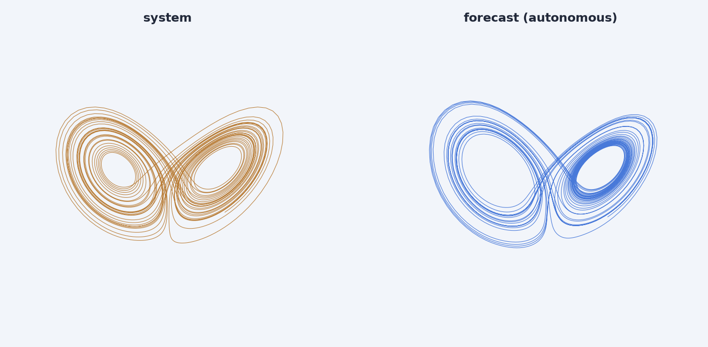
If forecasts diverge well before this point, tune the hyperparameters before increasing reservoir size. To quantify how far a forecast tracks — and to report it in the hardware- and system-independent unit of Lyapunov times — see Work · Lyapunov time.

Locking the forecast — golden regression fixtures

The forecast path is the library's most-revised code, so its behaviour is pinned by committed golden trajectories. For every forecast-capable premade model (classic_esn, ott_esn, power_augmented) plus an NG-RC forecaster, a fully-seeded warmup → forecast on a canonical Lorenz-63 series is checked in under tests/fixtures/golden_forecast/ and asserted by tests/test_models/test_golden_forecast.py:

• the first forecast steps must match the golden within a tight tolerance — the structural guard that catches any silent shift in the autoregressive loop (slot-0, the warmup/forecast seam, the flat single-step engine);
• the Valid Prediction Time against the true continuation must clear a committed floor — a coarser "forecast quality didn't collapse" guard.

If you intentionally change the forecast path (or the canonical data generators), regenerate the goldens and review the diff:

python tools/regen_golden_forecasts.py --check   # verify only — write nothing (CI-style drift check)
python tools/regen_golden_forecasts.py --all     # rewrite every fixture

Next

• Lyapunov time — score forecast quality and report horizons in Lyapunov times
• Tune — hyperparameter optimization for forecast quality
• Theory · Timing — derivation of every index in the forecast loop