Start · 02

First forecast

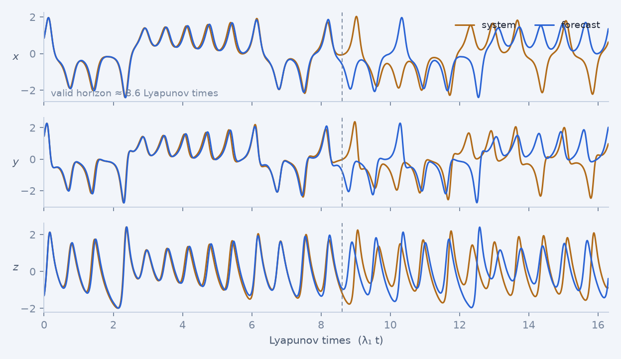
The script below trains a 900-neuron reservoir on five thousand samples of the Lorenz attractor, then forecasts two thousand steps autoregressively, feeding each prediction back as the next input. Training is a single algebraic solve; there is no gradient-descent loop.

import torch
import resdag as rd

# --- A chaotic system to learn: Lorenz-63, integrated with Euler steps ---
def lorenz(n, dt=0.01):
    xyz = torch.tensor([1.0, 1.0, 25.0])
    out = torch.empty(n, 3)
    for i in range(n):
        x, y, z = xyz
        xyz = xyz + dt * torch.tensor([10 * (y - x), x * (28 - z) - y, x * y - 8 / 3 * z])
        out[i] = xyz
    return out.unsqueeze(0)                    # (batch=1, time, 3)

data = lorenz(7500)
data = (data - data.mean(1, keepdim=True)) / data.std(1, keepdim=True)

# --- Split the timeline into warmup / train / validation segments ---
warmup, train, target, f_warmup, val = rd.utils.prepare_esn_data(
    data, warmup_steps=300, train_steps=5000, val_steps=2000
)

# --- Build, train, forecast ---
model = rd.models.ott_esn(reservoir_size=900, feedback_size=3, output_size=3)

rd.ESNTrainer(model).fit(
    warmup_inputs=(warmup,),
    train_inputs=(train,),
    targets={"output": target},
)

prediction = model.forecast(f_warmup, horizon=2000)    # (1, 2000, 3)

All three Lorenz components, true system against autonomous ESN forecast. The dashed line marks the valid horizon — about 8–9 Lyapunov times here, from the same 900-unit model after a small grid search over spectral radius and ridge alpha. Divergence past that point reflects the chaotic sensitivity of the system, not a defect in the model.

---

What each block did

The split. prepare_esn_data cuts one timeline into everything the workflow needs:

[ warmup │ train ────────────────────── │ val ]
                          └─ f_warmup ─┘

target is train shifted forward one step — the model learns given the signal now, emit the signal one step ahead. f_warmup is the tail of train, used to re-synchronize the reservoir immediately before the held-out window. Normalization is important: the tanh activation saturates when inputs are far from order one.

The model. ott_esn wires the architecture Pathak et al. used for chaotic systems: a frozen random reservoir, a quadratic state augmentation, and a ridge-regression readout named "output". The reservoir weights stay fixed; training changes only the readout's linear map.

The fit. One teacher-forced pass over warmup synchronizes the state; one pass over train collects states and solves the ridge problem against target by conjugate gradient. The "output" key in targets matches the readout's name parameter; this is how target tensors are routed to readout layers.

The forecast. Two phases: teacher-forced warmup on f_warmup, then horizon autoregressive steps where each output becomes the next input. The returned tensor aligns one-to-one with val, so the forecast error can be computed directly.

If the forecast diverges early

Adjust spectral_radius (0.8–1.2) and the readout's alpha (log-scale, 1e-8–1e-2) first. The full set of tuning parameters is covered in Tune.

Next

03 · The mental model — the four ideas everything else builds on.